Download
1 / 24
240 likes | 255 Views
Cloud Detection. 1) Optimised CI Microwindows cnc 2) Singular Vector Decomposition 3) Comparison of Methods fffffffffff. 1) CI Microwindow Optimisation. Currently: MW1 = [788.2, 796.25] cm -1 MW2 = [832.3, 834.4] cm -1 CI = L MW1 / L MW2 If CI < threshold → cloud

E N D
Cloud Detection 1) Optimised CI Microwindowscnc 2) Singular Vector Decomposition 3) Comparison of Methods fffffffffff
Currently: MW1 = [788.2, 796.25] cm-1 MW2 = [832.3, 834.4] cm-1 CI = LMW1 / LMW2 If CI < threshold → cloud If CI > threshold → clear operational threshold = 1.8 CRISTA experiment Aim: Find a better pair of MWs, and/or a better threshold value, using objective criteria based on simulated spectra with known cloud amounts
Spectral database: Tangent Height: 6, 9, 12, 15, 18, 21 km Cloud-Top Height: -2,-1.5,-1,-0.5,0,0.5,1.0,1.5,2.0 Cloud extinction: 0.1, 0.01, 0.001/km Atmospheres: mid-lat night, equatorial day, polar winter (night) and polar summer (day), plus these perturbed by 1-sigma climatological variations (Remedios, 2001) A TOTAL OF 1296 CLOUDY ATMOSPHERES REPRESENTED
Cloud Effective Fraction CEF: where k is the cloud extinction (/km), x is the integrated distance along a pencil beam within the cloud, is the normalised field-of-view response function, z is the tangent height ‘CLOUD DETECTION’ REDUCED TO PARTICULAR THRESHOLD VALUE OF CEF
Best MWs are those which best correlate CI with CEF … Current MWs show ~ linear relationship: for a,b minimumizing
Iterative approach (Desmond): Search through MWs with integer wavenumber boundaries and then, for each 'coarse' MW, iterate moving each boundary one grid point at a time. MW1 MW2 RMSE Current MWs [788.2, 796.25] [832.3, 834.4] 0.181 Optimised MWs [774.075, 775.0] [819.175, 819.95] 0.157
MW1 = [777, 779] cm-1 MW2 = [819, 820] cm-1 RMSE = 0.156 Monte-Carlo approach: Randomly-selecting MWs from the domain (specified by mid-point and width) and iterating from these to adjust the boundaries 10000 different MW pairs randomly selected from the entire 750–970 cm-1. Select region of lowest RMSE and do another 10000 iterations. Repeat.
Another criterion: Best MWs will have large relative distance between clear and cloudy distributions of CI RelDist = (mean CIclear – mean CIcloudy) / (stddevclear + stddevcloud)
MW1 = [800, 802] cm-1 MW2 = [831, 832] cm-1 RelDist = 2.77 Current MWs have RelDist = 2.03
Summary and Future Work MW1 MW2 RMSE RelDist Current MWs [788.2, 796.25] [832.3, 834.4] 0.181 2.03 Desmond MWs [774.075, 775.0] [819.175, 819.95] 0.157 na M.C. RMSE MWs [777.0, 779.0] [819.0, 820.0] 0.156 na M.C. RelDist MWs [800.0, 802.0] [831.0, 832.0] na 2.77 • In future: • Iterate within M.C MWs to find exact location of min/maximum • See how the two agree • Test to see how rigorous each set of MWs is at cloud detection and EF estimation
Singular Vector Decomposition SVD: • is statistical technique used for finding patterns in high dimensional data: • m×n matrix A can be decomposed into • A=V DU • V m×m left-singular vectors • U m×n right-singular vectors • D m×m singular values • transforms a number of potentially correlated variables into a smaller number of uncorrelated variables (SINGULAR VECTORS) orthonormal matrices diagonal matrix
In this case: A is a set of m spectra each of length n Each row of U is a singular vector with n ‘spectral points’ Singular value Dii weights the Uj singular vector. Idea is to find singular vectors that describe clear and cloudy atmospheres and use them in cloud detection
Use SVclear and SVcloud to do a Least Squares Fit of arbitrary signal L(ϑ) = ∑Ni ci SVclear i + ∑Mj dj SVclear j 15km 12km 9km 6km
1, then clear >1, then cloud Chi-Squared Ratio Test: , and then threshold
0, then clear 1, then cloud , and then threshold total Integrated Radiance Ratio Test:
Summary and Future Work: • Have successfully calculated SVs to represent atmospheric constituent variability (SVclear) and SVs to capture variability in cloud spectra (SVcloud) • Have implemented two detection methods and have defined thresholds using simulated and real MIPAS data • Have tested proficiency using simulated data • Complete full comparison of different cloud detection methods used to date.
Comparison of Detection Methods: 1. Current Operational CI 2. Optimised CI microwindows 3. SVD chi-squared ratio 4. SVD integrated radiance ratio 5. Simple radiance threshold Idea: Compare retrievals (using MORSE) of 'well-mixed' gases assuming that using spectra with residual cloud will result in retrievals which deviate significantly from climatology
Analysis done on cases where: Different cloud-detection methods disagree over whether it is clear/cloudy – and only use the clear cases
Summary and Future Work • Std. Deviations in VMRs from climatological means for retrieved well-mixed trace gases from MORSE should give measure of strength of each detection method • No clear ‘winner’ yet • Continue testing and comparing … CIRA climatology??