Download
1 / 45
470 likes | 667 Views
Lecture 3 : Direct Volume Rendering. Bong-Soo Sohn School of Computer Science and Engineering Chung-Ang University. Acknowledgement : Han-Wei Shen Lecture Notes 사용. Direct Volume Rendering. Direct : no conversion to surface geometry Four methods Ray-Casting Splatting

E N D
Lecture 3 : Direct Volume Rendering Bong-Soo Sohn School of Computer Science and Engineering Chung-Ang University Acknowledgement : Han-Wei Shen Lecture Notes 사용
Direct Volume Rendering • Direct : no conversion to surface geometry • Four methods • Ray-Casting • Splatting • 3D Texture-Based Method • CUDA
Data Representation • 3D volume data are represented by a finite number of cross sectional slices (hence a 3D raster) • On each volume element (voxel), stores a data value (if it uses only a single bit, then it is a binary data set. Normally, we see a gray value of 8 to 16 bits on each voxel.) N x 2D arraies = 3D array
A voxel is a cubic cell, which has a single value cover the entire cubic region A voxel is a data point at a corner of the cubic cell The value of a point inside the cell is determined by interpolation Data Representation What is a Voxel? – Two definitions
Basic Idea Based on the idea of ray tracing • Trace from eat each pixel as a ray into object space • Compute color value along the ray • Assign the value to the pixel
Transfer Function Maps voxel data values to optical properties Color/opacity map Emphasize or classify features of interest in the data Piecewise linear functions, Look-up tables, 1D, 2D GPU – simple shader functions, texture lookup tables
Viewing • Ray Casting • Where to position the volume and image plane • What is a ‘ray’ • How to march a ray
E0 u0 E v v0 u + S0 S (0,0,0) x y z Viewing B = [0,0,0] S0 = [0,0,-D] u0 = [1,0,0] v0 = [0,1,0] B Now, R: the rotation matrix S = B – D x g U = [1,0,0] x R V = [0,1,0] x R
Ray Casting • Stepping through the volume: a ray is cast into the volume, sampling the volume at certain intervals • The sampling intervals are usually equi-distant, but don’t have to be (e.g. importance sampling) • At each sampling location, a sample is interpolated / reconstructed from the grid voxels • popular filters are: nearest neighbor (box), trilinear (tent), Gaussian, cubic spline • Along the ray - what are we looking for?
Basic Idea of Ray-casting Pipeline • Data are defined at the corners • of each cell (voxel) • The data value inside the • voxel is determined using • interpolation (e.g. tri-linear) • Composite colors and opacities • along the ray path • Can use other ray-traversal schemes as well c1 c2 c3
Ray Traversal Schemes Intensity Max Average Accumulate First Depth
Ray Traversal - First • First: extracts iso-surfaces (again!)done by Tuy&Tuy ’84 Intensity First Depth
Ray Traversal - Average • Average: produces basically an X-ray picture Intensity Average Depth
Ray Traversal - MIP • Max: Maximum Intensity Projectionused for Magnetic Resonance Angiogram Intensity Max Depth
Ray Traversal - Accumulate • Accumulate opacity while compositing colors: make transparent layers visible!Levoy ‘88 Intensity Accumulate Depth
1.0 Raycasting volumetric compositing color opacity object (color, opacity)
Raycasting Interpolationkernel volumetric compositing color opacity 1.0 object (color, opacity)
1.0 Raycasting Interpolationkernel volumetric compositing color c = c s s(1 - ) + c opacity = s (1 - ) + object (color, opacity)
Raycasting volumetric compositing color opacity 1.0 object (color, opacity)
Raycasting volumetric compositing color opacity 1.0 object (color, opacity)
Raycasting volumetric compositing color opacity 1.0 object (color, opacity)
Raycasting volumetric compositing color opacity 1.0 object (color, opacity)
Raycasting volumetric compositing color opacity object (color, opacity)
Volume Ray Marching Raycast – once per pixel Sample – uniform intervals along ray Interpolate – trilinear interpolate, apply transfer function Accumulate – integrate optical properties
Shading and Classification • - Shading: compute a color(lighting) for each data point in the • volume • - Classification: Compute color and opacity for each data point • in the volume • Done by table lookup (transfer function) f(xi) C(xi), a(xi)
Shading (Local Illumination) Resulting = Ambient + Diffuse + Specular • Blinn-Phong Shading Model • Requires surface normal vector • What’s the normal vector of a voxel? Gradient • Central differences between neighboring voxels
Shading (Local Illumination) • Compute on-the-fly within fragment shader • Requires 6 texture fetches per calculation • Precalculate on host and store in voxel data • Requires 4x texture memory • Pack into 3D RGBA texture to send to GPU
Shading (Local Illumination) Improve perception of depth Amplify surface structure
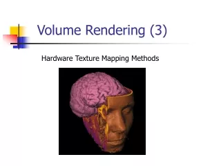
3D Texture Based Volume Rendering • Best known practical volume rendering method for rectlinear grid datasets • Realtime Rendering is possible
Interpolation of Samples • Volume stored as 3D texture • Viewport-aligned slices • Blended back-to-front • Trilinear interpolation by hardware
Classification • Density values from texture map • Classification via lookup table • Takes place in texture mapping stage
Shading is possible • Principle • Precompute Gradient plus density in texture • Shade first intensity (keep density!) • Classification via 2D pixel texture
Texture Mapping + Textured-mapped polygon 2D image 2D polygon
Texture Mapping for Volume Rendering Consider ray casting … (top view) z y x
Texture based volume rendering z y x Use pProxy geometry for sampling • Render every xz slice in the volume as a texture-mapped polygon • The proxy polygon will sample the volume data • Per-fragment RGBA (color and opacity) as classification results • The polygons are blended from back to front
Changing Viewing Direction y x What if we change the viewing position? That is okay, we just change the eye position (or rotate the polygons and re-render), Until …
Solution Use Image-space axis-aligned slicing plane: the slicing planes are always parallel to the view plane
Shading Use per-fragment shader Store the pre-computed gradient into a RGBA texture Light 1 direction as constant color 0 Light 1 color as primary color Light 2 direction as constant color 1 Light 2 color as secondary color
CUDA Volume Rendering • Utilize massively parallel computing resources • Assign each CUDA thread deal with a single ray • CUDA • Suitable for computing lots of independent work (e.g. processing pixels or voxels)