Download
1 / 21
210 likes | 234 Views
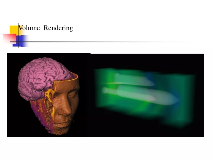
Volume Rendering. Scalar Data Visualization. Isosurface Extraction: extract geometry first, then render the resulting polygons (2) Volume Rendering: Direct display method project each data point onto the screen 2). Early attempts (pre-MCs).

E N D
Scalar Data Visualization • Isosurface Extraction: • extract geometry first, • then render the resulting • polygons • (2) Volume Rendering: • Direct display method • project each data point onto • the screen • 2)
Early attempts (pre-MCs) The Cuberille Approach (1979) - Each voxel has a value - Each voxel has 6 faces - Applying a threshold to perform binary classification - Draw the visible faces of the boundary voxels as polygons (Fairly jagged images) voxel
Contour Tracking Extract contours at each section and connect them together (1976 and after)
New Methods Were Needed Better image quality is necessary Finding object’s boundary sometimes can be difficult) The process of connecting boundary contours is also very complicated The intermediate geometry size can be huge
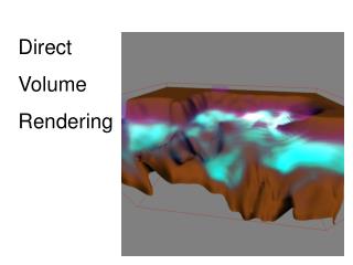
Direct: No conversion from data to geometry Direct 2-D Display of 3D Objects Tuy and Tuy 1984, IEEE CG & A (one of the earliest volume rendering techniques)
Basic Idea Based on the idea of ray tracing • Treat each pixel as a • light source • Emit light from the image • to the object space • The ray stops at the • object boundary • Calculate shading at • the boundary point • Assign the value to the • pixel
Algorithm details • Data Representation: (establish 3D • volume and 2D screen space) • Viewing • Sampling • Shading
Data Representation 3D volume data are represented by a finite number of cross sectional slices (a stack of images) N x 2D arraies = 3D array
A voxel is a cubic cell, which has a single value cover the entire cubic region A voxel is a data point at a corner of the cubic cell The value of a point inside the cell is determined by interpolation Data Representation (2) What is a Voxel? – Two definitions
Viewing • Ray Casting • Where to position the volume and image plane • What is a ‘ray’ • How to march a ray
Viewing (1) 1. Position the volume Assuming the volume dimensions is w x w x w We position the center of the volume at the world origin Volume center = [w/2,w/2,w/2] (local space) Translate T(-w/2,-w/2,-w/2) (0,0,0) x (data to world matrix? world to data matrix ) y z
(0,0,0) x y z Viewing (2) 2. Position the image plane Assuming the distance between the image plane and the volume center is D, and initially the center of the image plane is (0,0,-D) Image plane
Viewing (3) 3. Rotate the image plane A new position of the image plane can be defined in terms of three rotation angle a,b,g with respect to x,y,z axes Assuming the original view vector is [0,0,1], then the new view vector g becomes: cosb 0 -sinb 1 0 0 cosg sing 0 g = [0,0,1]0 1 0 0 cosa sina -sing cosg 0 sinb 0 cosb 0 -sina cosa 0 0 1
E0 u0 E v v0 u + S0 S (0,0,0) x y z Viewing (4) B = [0,0,0] S0 = [0,0,-D] u0 = [1,0,0] v0 = [0,1,0] B Now, R: the rotation matrix S = B – D x g U = [1,0,0] x R V = [0,1,0] x R
Viewing (5) Image Plane: L x L pixels Then E = S – L/2 x u – L/2 x v So Each pixel (i,j) has coordinates P = E + i x u + j x v S + v u E R: the rotation matrix S = B – D x g U = [1,0,0] x R V = [0,1,0] x R We enumerate the pixels by changing i and j (0..L-1)
d p x x x x Q Viewing (6) 4. Cast rays Remember for each pixel on the image plane P = E + i x u + j x v and the view vector g = [0,0,1] x R So the ray has the equation: Q = P + k (d x g) d: the sampling distance at each step K = 0,1,2,…
Sampling At each step of the ray, we sample the volume data What do you mean ?
Sampling (1) Q = P + K x V (v=dxg) At each step k, Q is rounded off to the nearest voxel (like the DDA algorithm) Check if the voxel is on the boundary or not (compare against a threshold) If yes, perform shading In tuys’ paper
Shading • Take the voxel position, distance to the image plane, the • object normal, and the light position into account • The paper does not describe in detail, but you can imagine • we can easily perform local illumination (diffusive or • even specular). • The distance can be used alone to provide • An 3D depth cue (e.g. distant voxels are dimmer)
Pros and Cons + Require no boundary estimation/hidden surface removal + No display holes - Binary object representation - Flat lighting (head on illumination) - Jagged surface - No semi-transparencies A more sophisticated classification and lighting model in [Levoy 88]