Volume Rendering

1. Volume Rendering Volume Modeling Volume Rendering 20 Apr. 2000

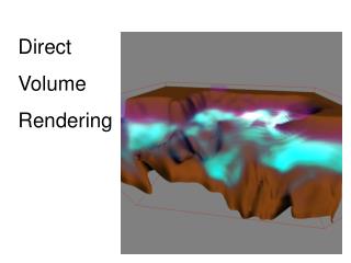
2. Volume Modeling & Rendering • Some data is more naturally modeled as a volume, not a surface • You could always convert the volume to a surface, but that’s not always best • Volume rendering: render the volume directly Ray-traced isosurface f(x,y,z)=c Same data, rendered as a volume

3. Why Bother with Volume Rendering? • Isn’t surface modeling & rendering easier? • Show all your data • more informative • less misleading (the isosurface of noisy data is unpredictable) • Constructive Solid Geometry (CSG) is natural • Simpler and more efficient than converting a very complex data volume (like the inside of someone’s head) to polygons and then rendering them

4. Surface Rendering Surface rendering is the "usual" type of rendering. Data is converted to geometrical primitives (e.g. triangles), which are then drawn. Everything you see is a 2D surface, embedded in a 3D space. The conversion to geometrical primitives may lose or disguise some data. Good for opaque objects, objects with smooth surface. Volume Rendering Data consists of one or more (supposedly continuous) fields in 3D. A Transfer Function maps the data into a volume of RGBA values. This volume is rendered directly, like a blob of colored jello. Data is seen more directly; less likely to be hidden. Works well for complex surfaces. Contrasts

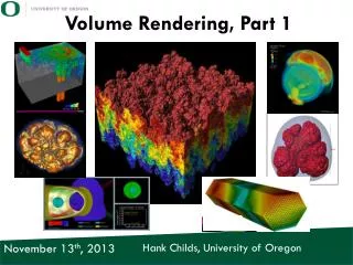
5. Applications • medical • Computed Tomography (CT) • Magnetic Resonance Imaging (MRI) • Ultrasound • engineering & science • Computational Fluid Dynamics (CFD) – aerodynamic simulations • meteorology – weather prediction • astrophysics – simulate galaxies • Computer Graphics • Participating media • Texels

6. Brief History of Volume Visualization • 1970’s modeling & rendering with 3-D grids and octrees • 1984 ray casting volume models • 1986 3-D scan conversion of lines, polygons into 3-D grid • 1987 marching cubes algorithm (convert volume model to surface model) • 1988 direct volume rendering with painter’s algorithm • 1989 splatting • 1990’s volume rendering hardware

7. Volume Rendering Pipeline • Data volumes come in all types: tissue density (CT), relaxation time of certain molecules (MRI), windspeed, pressure, temperature, value of implicit function. • Data volumes are used as input to a transfer function, which produces a sample volume of colors and opacities as output. • Typical might be a 256x256x64 CT scan • That volume is rendered to produce a final image. transfer function sample volume rendering final image data volumes

8. Transfer Functions • The transfer function takes (multiple) scalar data values as input, and outputs RGBA • It gets applied to every voxel in the volume “model” • It can be very simple (a color lookup table) or very complicated (implementing CSG, voxel texturing, etc.)

9. Rendering • Usually one just integrates color through the volume (ray casting) • Recursive ray tracing is also possible • But it gets confusing pretty quickly (shadows, filtered light, reflections, etc) • For lighting we need surfaces! • We can use the magnitude of the local gradient to check for surfaces (for example, bone is denser than fat on CT scans) • And we can use the (negative of the) gradient direction as a lighting normal! • Some, all, or none of the voxels will have surface lighting. • And we need material properties! • Either assume all the data is one material type, • Or use a separate set of segmentation data to identify voxel materials.

10. Some Details • Regular x-y-z data grids are easiest and fastest to handle, but algorithms exist for handling irregular grids like finite element models, where the voxels (volume elements) are not all parallelepipeds. • Resample it • or just deal with it • Finite element data, ultrasound data • Geometrical primitives can be handled by "rasterizing" them into data grids. This model was rasterized and rendered with VolVis

11. Accumulating Opacity • By convention, opacity (alpha) ranges from 0.0 to 1.0, 1.0 being completely opaque. • Multiple layers of material are composited according to their opacity. • An ideal, continuous material takes the limit of this process as it goes to an infinite number of infinitely thin layers (exponentials). • The local gradient of opacity can be used to detect surfaces, and as the normal for the lighting equation.

12. Ray Casting Volumes • Just integrate color and opacity along the ray • Simplest scheme just takes equal steps along ray, sampling opacity and color • Grids make it easiest to find the next cell • It’s simple to include volumes as primitives in a ray tracer • clouds, fog, smoke, fire done this way

13. Trilinear Interpolation • How do you compute RGBA values which are not at sample points? • Nearest neighbor (point sampling) yields blocky images • Trilinear interpolation is better, but slower • Just like texture mapping • You can even mipmap in 3D Nearest Neighbor Trilinear Interpolation

14. Splatting • Wonderfully simple • Working back-to-front (or front-to-back), draw a “splat” for each chunk of data • Easy to implement, but not as accurate as ray casting • works reasonably for non-gridded data closeup of a splat

15. Other Techniques • Shear-Warp (Lacroute and Levoy) • requires a grid • sort of like Bresenham for volumes • very fast with no hardware acceleration, but implementation is tricky • Polygons + 3D texture • Build a 3D texture, including opacity • Draw a stack of polygons from back to front, with that texture • Very efficient on machines with hardware acceleration that supports opacity 3D RGBA Texture Viewpoint Draw polygons back to front

16. head CSG is Easy • The transfer function can be used to mask a volume or merge volumes • You are still confined to the grid, of course not and or

17. Another CSG example (VolVis again)

18. Acceleration Techniques • Limit yourself to what you can do in cache... • …and do multiple blocks if necessary • Octrees • Quit integration early- that last bit is slowest • Error measures • Parallelism

19. Pictures colliding galaxies