Download
1 / 42
420 likes | 543 Views
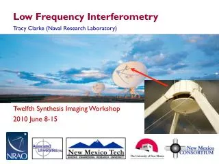
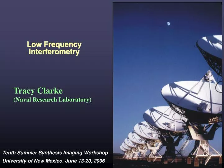
Low Frequency Interferometry. Tracy Clarke (Naval Research Laboratory). History of Radio Astronomy: Low Frequencies. Jansky. Reber. Radio astronomy was born in the 1930's with Karl Jansky's work at 20.5 MHz (14.5 m) at Bell labs Reber continued radio astronomy work at 160 MHz (1.9 m).

E N D
Low Frequency Interferometry Tracy Clarke (Naval Research Laboratory)
History of Radio Astronomy: Low Frequencies Jansky Reber • Radio astronomy was born in the 1930's with Karl Jansky's work at 20.5 MHz (14.5 m) at Bell labs • Reber continued radio astronomy work at 160 MHz (1.9 m)
History of Radio Astronomy ~ 1’, rms ~ 3 mJy/beam ~ 10’, rms ~ 30 mJy/beam • First radio telescopes operated at long wavelengths with low spatial resolution and very high system temperatures • Radio astronomy quickly moved to higher frequencies with better spatial resolution ( ) and lower system temperatures
Science: Thermal vs. Synchrotron Emission Thermal Emission (Free-Free, Bremsstrahlung): • Best observed at cm GHz) • Deflection of free electrons by positive ions in hot gas • Depends on temperature of the gas Synchrotron Emission: • Best observed at m GHz) • Relativistic electrons spiraling around magnetic field lines (high-energy astrophysics) • Depends on the energy of the electrons and magnetic field strength • Emission is polarized • Can be either coherent or incoherent Synchrotron Synchrotron self absorption or free-free absorption Thermal: Rayleigh-Jeans Thompson, Moran, & Swenson
Bursts From Jupiter & Extra-Solar Planets VLA 74 MHz Jupiter images • Jupiter's coherent cyclotron emission: complex interaction of Jupiter’s magnetosphere with Io torus POSSIBLE TO DETECT BURST EMISSION FROM DISTANT “JUPITERS” Bastian et al. VLA SYSTEM CAN DETECT QUIESCENT EMISSION Future instrumentswill resolve Jupiter and may detect extra-solar planets
Galactic Science Examples • Galactic: - Galactic center black hole Sgr A* - non-thermal filaments: magnetic field orientation - transients - supernova remnant census - SNR acceleration - HII regions - diffuse nonthermal source (DNS): field strength
Galactic Center Filaments • Galactic Center: non-thermal filaments • Synchrotron filaments trace magnetic field lines and particle distribution. • Near the Galactic center filaments are perpendicular to the plane but the “Pelican” filament is parallel to the plane, allowing the magnetic field orientation to be further mapped Lang et al. (1999)
Transients GCRT J1745-3009 ~10 minute bursts every 77 minutes – timescale implies coherent emission Coherent GC bursting source • Transients: sensitive, wide fields at low frequencies provide powerful opportunity to search for new transient sources • candidate coherent emission transient recently discovered near Galactic center (Hyman, et al., 2005, Nature)
Galactic Supernova Remnant Census • Census: expect over 1000 SNR and know of ~230 330 MHz 8 m 2 Color Image: Red: MSXat 8 m Blue: VLA 330 MHz Tripled (previously 17, 36 new) known SNRs in survey region! Brogan et al. (2006)
SNRs: Shock Acceleration vs.Thermal AbsorptionCas A 74/330 Spectral Index A array + Pie Town A array (T. Delaney – thesis with L. Rudnick)
Pulsars • Detecting fast (steep-spectrum) pulsars • highly dispersed, distant PSRs • tight binaries • submsec? • Probe PSR emission mechanism • explore faint end of luminosity function • spectral turnovers near 100 MHz • New SNR/pulsars associations -- Deep, high surface brightness imaging of young pulsars Erickson 1983 Crab Nebula & pulsar @ 74 MHz Spectrum of 4C21.53: 1st msec pulsar
Extragalactic Science Examples • Extragalactic: - radio galaxy lifecycle - particle acceleration in radio galaxies - radio lobe particle content - energy feedback into the intracluster medium - particle acceleration in merger/accretions shocks - tracing Dark Matter - sample selection for Dark Energy studies - detection of high redshift radio galaxies - study of epoch of reionization
Radio Galaxies: Outburst Lifecycle • Hydra A at 4500 MHz (inset) shows an FR-I morphology on scales of <1.5' (100 kpc) • New 74 and 330 MHz data show Hydra A is > 8' (530 kpc) in extent with large outer lobes surrounding the high frequency source • Outer lobes have important implications for the radio source lifecycle and energy budget -12000 Lane et al. (2004)
Driving Shocks into the ICM • Chandra X-ray emission detects shock front surrounding low frequency radio contours • Expanding radio lobes drive the shock over last ~1.4x10⁸ yr • Total energy input significantly exceeds requirements to offset X-ray cooling in cluster Nulsen et al. (2005)
Galaxy Cluster Cores: AGN Feedback 74 MHz 330 MHz Fabian et al. (2002)
Cluster Mergers: Diffuse Synchrotron Emission Several clusters display large regions of diffuse synchrotron: • 'halos' & 'relics' associated with merging clusters • radio emission is generally steep spectrum • location, morphology, spectral properties, etc... can be used to understand merger geometry Abell 2256 Clarke & Ensslin (2006)
Cosmology: Tracing Dark Energy Observations of cosmic acceleration have led to studies of Dark Energy: • clusters should be representative samples of the matter density in the Universe • study DE through various methods including the 'baryonic mass fraction' • requires assumption of hydrostatic equilibrium • merging cluster can be identified and removed using low frequency detections of halos and relics (Clarke et al. 2005) Allen et al. (2004)
High Redshift Galaxies: Steep Spectrum THEORETICAL SYNCHROTRON AGING SPECTRA (KARDASHEV-PACHOLCZYK MODEL) 2 0 log S INCREASING REDSHIFT -2 -4 -4 -3 -2 -1 0 1 2 log [GHz] Observations of cosmic acceleration have led to studies of Dark Energy: • Synchrotron losses steepen the spectrum of radio galaxies at high z • Inverse Compton losses act similarly to steepen the spectrum, especially at high z since IC losses scale as z4. • Spectrum is also red shifted to lower frequencies so that the entire observed spectrum is steep.
Epoch of Reionization: z 6 (H I at 200 MHz) Universe made rapid transition from largely neutral to largely ionized • Appears as optical Gunn-Peterson trough in high-z quasars • Also detectable by highly-red shifted 21 cm H I line in absorption against first quasars, GRB’s, SF galaxies … • WMAP 3yr: re-ionization epochs near z~11 (HI at 115 MHz) SDSS: Becker et al. (2001)
VLA Low Frequency Sky Survey: VLSS • Survey Parameters • 74 MHz • Dec. > -30 degrees • 80” resolution • rms ~100 mJy/beam • Deepest & largest LF survey • N ~ 105 sources in ~ 80% of sky • Statistically useful samples of rare sources => fast pulsars, distant radio galaxies, cluster radio halos and relics • Unbiased view of parent populations for unification models • Important calibration grid for VLA, GMRT, & future LF instruments • Data online at: http://lwa.nrl.navy.mil/VLSS • Condon, Perley, Lane, Cohen, et al ~ 95 % complete
VLSS FIELD 1700+690 ~80”, rms ~50 mJy ~20o
Low Frequency In Practice: Not Easy! • Bandwidth smearing Distortion of sources with distance from phase center • Interference: Severe at low frequencies • Phase coherence through ionosphere Corruption of coherence of phase on longer baselines • Finite Isoplanatic Patch Problem: Calibration changes as a function of position • Large Fields of View: Perley lecture Non-coplanar array (u,v, & w) Large number of sources requiring deconvolution Calibrators
Bandwidth Smearing Freq. (MHz) BW (MHz) A-config. synth (“) Radius of PBFWHM (‘) MAX (‘) for 50% degradation 74 1.5 25 350 41 330 6.0 6 75 11 1.3 1420 50 1.4 15 Solution: spectral line mode (already essential for RFI excision) Rule of thumb for full primary beam targeted imaging in A config. with less than 10% degradation: 74 MHz channel width < 0.06 MHz 330 MHz channel width < 0.3 MHz 1420 MHz channel width < 1.5 MHz • Averaging visibilities over finite BW results in chromatic aberration worsens with distance from the phase center => radial smearing )x(synth ~ 2 => Io/I = 0.5 => worse at higher resolutions
Radio Frequency Interference: RFI • As at cm wavelengths, natural and man-generated RFI are a nuisance • Getting “better” at low freq., relative BW for commercial use is low • At VLA: different character at 330 and 74 MHz • 74 MHz: mainly VLA generated => the “comb” from 100 kHz oscillators • 330 MHz: mainly external • Solar effects – unpredictable • Quiet sun a benign 2000 Jy disk at 74 MHz • Solar bursts, geomagnetic storms are disruptive => 109 Jy! • Ionospheric scintillations in the late night often the worst • Powerful Solar bursts can occur even at Solar minimum! • Can be wideband (C & D configurations), mostly narrowband • Requires you to take data in spectral line mode • RFI can usually be edited out – tedious but “doable”
RFI Excision 35 km 12 km 3 km before after RFI environment worse on short baselines Several 'types': narrow band, wandering, wideband, ... Wideband interference hard for automated routines Example using AIPS tasks FLGIT, FLAGR Unfortunately, still best done by hand! Time Frequency AIPS: SPFLG
RFI Excision in Practice • Approach: averaging data in time and/or frequency makes it easier to isolate RFI, which averages coherently, from Gaussian noise, which does not • Once identified, the affected times/baselines can be flagged in the un-averaged dataset • Where to start? AIPS tasks: QUACK, SPFLG, TVFLG, UVPLT, UVFND, UVFLG, UVSUB, CLIP, FLGIT, FLAGR, ... • Stokes V can be helpful to identify interference signals before after
Ionospheric Structure: ~ 50 km > 5 km <5 km • Waves in the ionosphere introduce rapid phase variations (~1°/s on 35 km BL) • Phase coherence is preserved on BL < 5km • BL > 5 km have limited coherence times • Historically limited capabilities of low frequency instruments
Ionospheric Effects Wedge Effects: Faraday rotation, refraction, absorption below ~ 5 MHz (atmospheric cutoff) Wave and Turbulence Effects: Rapid phase winding, differential refraction, source distortion, scintillations Wedge: characterized by TEC = nedl ~ 1017 m-2 Extra path length adds extra phase L 2 TEC ~ L ~ * TEC Waves: tiny (<1%) fluctuations superimposed on the wedge ~ 50 km ~ 1000 km Waves Wedge VLA • The wedge introduces thousands of turns of phase at 74 MHz • Interferometers are particularly sensitive to difference in phase (wave/turbulence component)
Ionospheric Refraction & Distortion Refractive wander from wedge 1 minute sampling intervals • Both global and differential refraction seen. • Time scales of 1 min. or less. • Equivalent length scales in the ionosphere of 10 km or less.
Antenna Phase as a Function of Time Phase on three 8-km baselines Refractive wedge At dawn Scintillation ‘Midnight wedge’ Quiesence TIDs A wide range of phenomena were observed over the 12-hour observation => MYTH: Low freq. observing is better at night. Often daytime (but not dawn) has the best conditions
'Dealing' with the Ionosphere • Self-calibration models ionosphere as a time-variable antenna based phase: i(t) • Loop consisting of imaging and self-calibration • model improves and S/N for self-cal increases • Typical approach is to use a priori sky-based model such as NVSS, WENSS, or higher frequency source model (AIPS: SETFC, FACES, CALIB, IMAGR) - freezes out time variable refraction - ties positions to known sky-model • DOES NOT ALWAYS WORK – e.g. fails due to thermal absorption • This method assumes a single ionospheric solution applies to entire FOV - in reality the assumption is only valid over a smaller region but is probably ok if most of the flux is in the source of interest and only want small FOV
Isoplanatic Patch Assumption • Zernike polynomial phase screen • Developed by Bill Cotton (NRAO) • Delivers astrometrically correct images • Fits phase delay screen rendered as a plane in 3-D viewed from different angles Key handicaps: • Need high S/N—significant data loss under poor ionospheric conditions • Total flux should be dominated by point sources • Standard self-calibration sets single ionospheric solution across entire FOV:i(t) • OK if brightest source is the only target of interest in the field • Problems: differential refraction, image distortion, reduced sensitivity • Solution: selfcal solutions with angular dependence i(t) i(t, , ) • Problem mainly for 74 MHz A and B arrays New tools will be needed for next generation of instruments
Breakdown of Finite Isoplanatic Assumption Self-calibration Zernike Model Average positional error decreased from ~45” to 17” AIPS: VLAFM
Large Fields of View (FOV) I Noncoplanar baselines: (u,v, and w) Perley lecture • Important if FOV is large compared to resolution => in AIPS multi-facet imaging, each facet with its own synth • Essential for all observations below 1 GHz and for high resolution, high dynamic range even at 1.4 GHz • Requires lots of computing power and disk space • AIPS: IMAGR (DO3DIMAG=1, NFIELD=N, OVERLAP=2), CASA (aka AIPS++): w-projection Example: VLA B array 74 MHz: ~325 facets A array requires 10X more: ~ 3000 facets ~108 pixels
Targeted Faceting Fly’s Eye ~ 4 degrees A array requires ~10,000 pixels! Outliers AIPS Tip: • Experience suggests that cleaning progresses more accurately and efficiently if EVERY facet has a source in it. • Best not to have extended sources spread over too many facets => often must compromise • enormous processing required to image entire FOV • reduce processing by targeting facets on selected sources (still large number!) • overlap a fly's eye of the central region and add individual outliers • AIPS: SETFC
Large Fields of View (FOV) II 1 Jy 9 Jy 330 MHz phase calibrator: 1833-210 Calibrators: • Antenna gain (phase and amplitude) and to a lesser degree bandpass calibration depends on assumption that calibrator is a single POINT source • Large FOV + low freq. = numerous sources everywhere • At 330 MHz, calibrator should dominate flux in FOV: extent to which this is true affects absolute positions and flux scale => Phases (but not positions) can be improved by self-calibrating phase calibrator => Always check accuracy of positions • Must use source with accurate model for bandpass and instrumental phase CygA, CasA, TauA, VirgoA
Amplitude and bandpass calibration: Cygnus A (few x 2 min) Blows through RFI! Phase calibration at 330 MHz: fairly easy Sky is coherent across the array in C and D configurations Observe one strong unresolved source anywhere in sky Traditional phase calibration in A and B arrays Now being superseded by NVSS Sky model – no phase calibration required! Phase calibration at 74 MHz: more challenging Cygnus A (or anything bright) is suitable in the C and D arrays A and B arrays: Cyg A works for initial calibration, because enough short spacings see flux to start self-cal process Selfcal can’t overcome breakdown of isoplanatic patch assumption Hourly scans on Cyg A => instrumental calibration for non-selfcal (Zernike polynomial) imaging Calibration schemes continue to evolve rapidly with time! Avoid Sun particularly in compact configurations VLA LF Observing Strategy
Current Low Frequency Interferometers: VLA • Two Receivers: 330 MHz = 90cm PB ~ 2.5O (FOV ~ 5O ) 74 MHz = 400cm PB ~ 12O (FOV ~ 14O ) • Simultaneous observations • Max 330 MHz resolution 6" (+PT resolution ~3") • Max 74 MHz resolution 25" (+PT resolution ~12")
74 MHz VLA: Significant Improvement in Sensitivity and Resolution 74 MHz VLA Many low frequency instruments in use!
Current Low Frequency Interferometers: GMRT 150 235 610 1420 327 50 • Five Receivers: 153 MHz = 190cm PB ~ 3.8O (res ~ 20" ) 235 MHz = 128cm PB ~ 2.5O (res ~ 12" ) 325 MHz = 90cm PB ~ 1.8O (res ~ 9" ) 610 MHz = 50cm PB ~ 0.9O (res ~ 5" )
For more information: Further reading: White Book: Chapters 12.2, 15, 17, 18, 19, & 29 From Clark Lake to the Long Wavelength Array: Bill Erickson's Radio Science, ASP Conference Series 345 Data Reduction: http://www.vla.nrao.edu/astro/guides/p-band/ http://www.vla.nrao.edu/astro/guides/4-band/ Future Instruments: LWA, LOFAR, MWA, FASR http://lwa.nrl.navy.mil, http://lwa.unm.edu(Taylor lecture) http://www.lofar.org/ Thanks to: C. Brogan (NRAO), N. Kassim, A. Cohen, W. Lane, J. Lazio (NRL), R. Perley, B. Cotton, E. Greisen (NRAO)