Download
1 / 12
120 likes | 329 Views
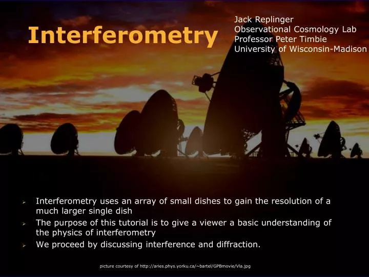
Interferometry. Jack Replinger Observational Cosmology Lab Professor Peter Timbie University of Wisconsin-Madison. Interferometry uses an array of small dishes to gain the resolution of a much larger single dish

E N D
Interferometry Jack Replinger Observational Cosmology Lab Professor Peter Timbie University of Wisconsin-Madison • Interferometry uses an array of small dishes to gain the resolution of a much larger single dish • The purpose of this tutorial is to give a viewer a basic understanding of the physics of interferometry • We proceed by discussing interference and diffraction. picture courtesy of http://aries.phys.yorku.ca/~bartel/GPBmovie/Vla.jpg
constructive interference destructive interference Two Slit Interference Interference pattern λ/2d light sources
detected in phase detected out of phase Two Slit Interference Reversed “Interference pattern” λ/2d The detectors are therefore sensitive to the interference pattern detectors
Adding Interferometer signal emitted from source reaches right antenna δt sooner than left antenna signal detected by right antenna delayed by δt such that at the tee, two corresponding signals are interfered diagram courtesy of http://www.geocities.com/CapeCanaveral/2309/page3.html
Antenna Optics • Antenna is designed such that parallel rays converge at focus • Use reversibility: Analogous to single slit diffraction
detectors sources total destructive interference undetectable maximum maximum response side lobe side lobe light source antenna Diffraction Reversed diffraction pattern λ/D The single antenna is therefore sensitive to the diffraction pattern
Two Slit Diffraction • Envelope due to antenna sensitivity (Diffraction) • Peaks due to baseline (Interference) • Angular Resolution (Rayleigh Criterion) is λ/2d from baseline, instead of λ/D from diffraction limit Image courtesy of http://img.sparknotes.com/figures/C/c33e2bffc162212e1d9aa769ad3ae54f/envelope.gif Image courtesy of http://www.ece.utexas.edu/~becker/diffract.pdf
contributes weak signal contributes strong signal contributes no signal Interferometer Sensitivity • Interferometer is like diffraction in reverse, in 2D • Each antenna is analogous to a circular aperture • Example at left is the Diffraction pattern from two circular apertures (shown at upper left) • The interferometer is sensitive to projection of the diffraction pattern on the sky • Sources in light regions are detected, signal strength varies with intensity • Sources in dark regions are undetectable courtesy of http://www.ee.surrey.ac.uk/Personal/D.Jefferies/aperture.html
P r θ 0- θ x xsinθ dx a- Fourier Analysis:Background • In order to understand how to reconstruct an image it is important to understand the mathematics of diffraction and interference • Notation: • x (and y) describe the plane of the aperture • θ (and Ф) describe the “plane” of the diffraction pattern Equation describing the E-field from a point source of the wave at any distance d E = Eoei(kd-wt)
P r θ 0- θ x xsinθ dx a- Fourier Analysis:Single Slit Diffraction at P, the electric field due to a small dx is dE = Eoei(k(r+xsinθ)-wt)dx at P, the electric field is E(θ) = ∫oaEoei(k(r+xsinθ)-wt)dx generally, for any aperture = Eo ∫aperture eikxsinθdx let A(x) describe the aperture = Eo ∫all space eikxsinθA(x)dx Generalizing this to two dimensions, and any aperture, the E field at P is E(θ,Ф) = Eo ∫all space eikxp+ikyq A(x,y)dxdy p and q are functions of θ and Ф, describing the phase shifts
P r θ 0- θ x xsinθ dx a- Fourier Analysis:Generalized Diffraction detector sky The intensity (proportional to E2) on the sky is therefore I(θ,Ф) = C*(E(θ,Ф))2 = C*(∫all space eikxp+ikyq A(x,y)dxdy)2 If the aperture is the detector, then the diffraction pattern describes the sensitivity of the instrument G(θ,Ф) = I(θ,Ф) The power P recorded by the detector is the product of the sensitivity function and the intensity of the sky S(θ,Ф) integrated over the sky P = ∫sky G(θ,Ф)*S(θ,Ф )dθdФ = C*∫sky(∫all spaceeikxp+ikyqA(x,y)dxdy)2*S(θ,Ф)dθdФ
P r θ 0- θ x xsinθ dx a- Fourier Analysis:Image Reconstruction detector sky P = C*∫sky(∫all spaceeikxp+ikyq A(x,y)dxdy)2*S(θ,Ф) dθdФ P is recorded each time the detector is pointed A(x) is determined by the aperture, p and q are known functions that describe the phase shifts By recording P and varying A, by changing the baselines or using multiple baselines if there are enough detectors, we obtain enough information to solve for S(θ,Ф) for that patch of the sky, fortunately this can be done on computers with existing software. For MBI the program will be written by Siddharth Malu. It is important to note that this is an oversimplification of the situation, when applying this is a diffuse source the coherence of the light from different regions of the source must be addressed with a coherence function. This is addressed by the Van Cittert-Zernike theorem, which is beyond the scope of this presentation.