Download
1 / 40
400 likes | 594 Views
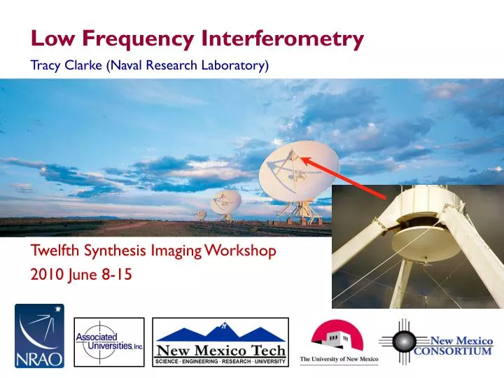
Low Frequency Interferometry. Tracy Clarke (Naval Research Laboratory). What is Low Frequency?. Wikipedia: ‘ Low frequency or low freq or LF refers to radio frequencies (RF) in the range of 30 kHz – 300 kHz.’. Not the definition normally used by radio astronomers.

E N D
Low Frequency Interferometry Tracy Clarke (Naval Research Laboratory)
What is Low Frequency? • Wikipedia: ‘Low frequency or low freq or LF refers to radio frequencies (RF) in the range of 30 kHz – 300 kHz.’ • Not the definition normally used by radio astronomers. • Low freq radio astronomy = HF (3 MHz – 30 MHz), VHF (30 MHz – 300 MHz) and UHF (300 MHz – 3 GHz) • Ground-based instruments only reach to ~10 MHz due to ionosphere
Jansky Low Frequencies: Origin of Radio Astronomy Reber • Radio astronomy was born in the 1930's with Karl Jansky's work at 20.5 MHz (14.5 m) at Bell labs • Reber continued work at 160 MHz (1.9 m) in his back yard
Reber Reber’s Radio Sky in 1944 • 160 MHz sky image from Reber, resolution ~12 degrees
Synchrotron Synchrotron self absorption or free-free absorption Thermal: Rayleigh-Jeans Emission Mechanisms at Low Frequency • Synchrotron Emission:(Lang Talk) • Best observed at m λ (ν < 1 GHz) • Relativistic electrons spiraling around magnetic field lines • Depends on the energy of the electrons and magnetic field strength • Emission is polarized • Can be either coherent or incoherent Thermal Emission: (Brogan Talk)(Free-Free, Bremsstrahlung): • Best observed at cm λ (ν > 1 GHz) • Deflection of free electrons by ions • Depends on temperature of the gas • Can be emission or absorption at low ν Thompson, Moran, & Swenson
Recombination Lines • Radio Recombination Lines: (Lang Talk) • High quantum number n state (n>100 for low frequencies), formed in transition region between fully ionized regions and neutral gas (PDRs) • Nomenclature: n+Δn→n, Δn=1 is nα, Δn=2 is nβ, νo∝Δn/n3(e.g. C441α) • Largely observed toward the Galactic Plane and discrete source. Detected in absorption below ~150 MHz. • Diagnostics of the physical conditions of the poorly probed cold ISM, e.g. temperature, density, level of ionization, abundance ratios • Frequency variable signal could adversely impact sensitive Dark Ages and Epoch of Reionization observations. Stepkin et al. (2007)
θ ~ 10’, rms ~ 30 mJy/beam θ ~ 1’, rms ~ 3 mJy/beam Fundamental Limitation • Spatial resolution depends on wavelength and antenna diameter: • First long wavelength antennas had very low spatial resolution • Astronomers pushed for higher resolution and moved to higher frequencies were the TSYS is also lower: (McKinnon Talk) Confusion:
Why ‘Abandon’ Low Frequencies? • Low frequency instruments had limited aperture due to ionosphere (B< 5 km) > 5 km <5 km • Confusion limit reached quickly with only short baselines • Imaging large fields of view posed enormous computing problem • Removal of radio frequency interference (RFI) was very difficult Correlation Preserved Correlation Destroyed
Overcoming the Resolution Problem • Currently in a transition of moving to high resolution at low frequenciesWhy has this taken nearly 50 years? • Software/Computing: • - Ionospheric decorrelation on baselines > 5 km is overcome by software advances of Self-Calibration in the 1980’s • - Wide-field imaging only recently (sort of) possible • - RFI excision development • - Data transmission from long distances became feasible using fiber-optic transmission lines
Recent advances in ionospheric calibration, widefield imaging, and RFI excision have led to a new focus on low frequency arrays Low Frequency Arrays ★ Dishes Dipoles Instrument Location ν range Resolution FoV Sensitivity (MHz) (arcsec) (arcmin) (mJy) VLA NM 73.8, 330 24-5 700-150 20-0.2 GMRT IN 151-610 20-5 186-43 1.5-0.02 WSRT NL 115-615 160-30 480-84 5.0-0.15 … LOFAR-Low NL 10-90 40-8 1089-220 110-12 LOFAR-Hi NL 110-250 5-3 272-136 0.41-0.46 LWA NM 10-88 16-1.8 16-1.6 1.0 ….. • ★ 330 MHz system not compatible with EVLA, 74 MHz system to be evaluated soon • – New receiver system under development
EVLA Low-Band ReceiverEvolution of Low-Frequency Capabilities on the VLA • 1983 P-Band (330 MHz) System Installed on the VLA • 1984 Pearson and Readhead introduce the self-calibration technique • 1991 Single 4-Band (74 MHz) Antenna Installed on the VLA • 1994 Eight 4-Band VLA Antennas • 1998 Full 4-Band VLA – All 27 Antennas (Ɵ ~ 25”) • 2002 Pie Town Link at 74 MHz (Ɵ ~ 8”) • 2008 P-Band system incompatible with EVLA electronics Twelfth Synthesis Imaging Workshop
EVLA Low-Band ReceiverDesign Goals for New Low-Frequency Receiver • Restore legacy low-frequency (LF) capabilities to EVLA • Improve sensitivity with lower receiver noise temperature • Marian Pospiezalski of NRAO CDL building P band amplifier • 4 band and spare channel amplifiers are commercial devices • Increase receiver bandwidth to enable future broadband feeds • Consolidation of LF capabilities into a single receiver subsystem • Provide an easily extensible platform for future LF feeds • Two completely independent “spare” channels provide • LNA –Ultra-Low Noise front end with high-dynamic range • Noise Calibration • Filter position to define a future frequency band • Upgrades to EVLA IF structure could enable frequency coverage from 50 MHz to 1 GHz Twelfth Synthesis Imaging Workshop
EVLA Low-Band ReceiverIncreased Bandwidth • 4-band: Increased from 1.5 MHz to ~16 MHz (66 to 82 MHz) • Limited on low end by present EVLA IF structure • Limited on high end by start of FM band (87.5 MHz) • P-band: Bandwidth increased from 40 MHz to 240 MHz (230 to 470 MHz) Twelfth Synthesis Imaging Workshop
EVLA Low-Band ReceiverConsolidated LF Platform to Enable Feed Development Power Supply Temperature Monitoring Noise Calibration Injection Combine Channels P-Band 230 – 470 MHz Broadband Linear Antenna Feeds XLP XLP XLP XLP YLP YLP YLP YLP 4-Band 66 – 82 MHz XLP Spare A TBD Exclusive of P-Band and 4-Band Coverage YLP Spare B TBD Exclusive of P-Band and 4-Band Coverage Twelfth Synthesis Imaging Workshop
Low Frequency Science • Key science drivers at low frequencies: • - Dark Ages (spin decoupling) • - Epoch of Reionization (highly redshifted 21 cm lines) • - Early Structure Formation (high z RG) • - Large Scale Structure evolution (diffuse emission) • - Evolution of Dark Matter & Dark Energy (Clusters) • - Wide Field (up to all-sky) mapping • - Large Surveys • - Transient Searches (including extrasolar planets) • - Galaxy Evolution (distant starburst galaxies) • - Interstellar Medium (CR, HII regions, SNR, pulsars) • - Solar Burst Studies • - Ionospheric Studies • - Ultra High Energy Cosmic Ray Airshowers • - Serendipity (exploration of the unknown)
Dark Ages EoR Dark Ages Loeb (2006) • Spin temperature decouples from CMB at z~200 (ν =7 MHz) and remains below until z~30 (ν =45 MHz) • Neutral hydrogen absorbs CMB and imprints inhomogeneities
Dark Ages EoR Epoch of Reionization Tozzi et al. (2000) • Hydrogen 21 cm line during EoR between z~6 (ν ~ 200 MHz) and z~11 (ν ~ 115 MHz) EoR Intruments: MWA, LOFAR, 21CMA, PAPER, SKA
Dark Ages EoR Structure Formation Clarke & Ensslin (2006) • Galaxy clusters form through mergers and are identified by large regions of diffuse synchrotron emission (halos and relics) • Important for study of plasma microphysics, dark matter and dark energy Structure Formation
4835 MHz 8465 MHz 330 MHz 1400 MHz Evolution of AGN Activity/Feedback X-ray residuals ? Clarke et al. (2005)
Galactic Supernova Remnant Census • Census: expect over 1000 SNR and know of ~230 330 MHz 8 μm MSX 2 Color Image: Red: MSXat 8 μm Blue: VLA 330 MHz Tripled (previously 17, 36 new) known SNRs in survey region! Brogan et al. (2006)
GCRT J1745-3009 Coherent GC bursting source ~10 minute bursts every 77 minutes – timescale implies coherent emission Transients: Galactic Center • Filaments trace magnetic field lines and particle distribution • Transients: sensitive, wide fields at low frequencies provide powerful opportunity to search for new transient sources • Candidate coherent emission transient discovered near Galactic center Hyman, et al., (2005) - Nature; Hyman et al. (2006, 2007) Lang et al. (1999)
VLA 74 MHz Jupiter images Extrasolar Planets • Jupiter's coherent cyclotron emission: complex interaction of Jupiter’s magnetosphere with Io torus POSSIBLE TO DETECT BURST EMISSION FROM DISTANT “JUPITERS” Bastian et al. VLA SYSTEM CAN DETECT QUIESCENT EMISSION • Future instrumentswill resolve Jupiter and may detect extra-solar planets
VLA Low Frequency Sky Survey: VLSS • Survey Parameters: ν = 74 MHz, δ > -30°, • Θ= 80” resolution, σ~100 mJy/beam • Deepest & largest LF survey • N ~ 70 000 sources in ~ 95% of sky > -30° • Statistically useful samples of rare sources • => fast pulsars, distant radio galaxies, cluster radio • halos and relics, unbiased view of parent • populations for unification models • Important calibration grid for EVLA, GMRT, & future LF instruments • Data online at NED & http://lwa.nrl.navy.mil/VLSS Cohen et al. (2007) Cohen et al. 2007, AJ, 134, 1245
VLSS FIELD 1700+690 θ~80”, rms ~50 mJy 19 ~20o
Low Frequency In Practice: Not Easy! • Phase coherence through ionosphere • Corruption of coherence of phase on longer baselines • Finite Isoplanatic Patch Problem: • Calibration changes as a function of position • Bandwidth smearing: • Distortion of sources with distance from phase center • Radio Frequency Interference: • Severe at low frequencies • Large Fields of View: • Non-coplanar array (u,v, & w) • Large number of sources requiring deconvolution • Calibrators
VLA + Pie Town outrigger (73 km) 74/330 MHz Spectral Index Not Easy but certainly possible! Delaney (2004) Lane et al. (2001)
Ionospheric Effects Wedge Effects: Faraday rotation, refraction, absorption below ~ 5 MHz (atmospheric cutoff) Wave and Turbulence Effects: Rapid phase winding, differential refraction, source distortion, scintillations Wedge: characterized by TEC = ∫nedl ~ 1017 m-2 Extra path length adds extra phase ΔL αλ2∗ TEC Δφ ~ ΔL⁄λ ~ λ * TEC Waves: tiny (<1%) fluctuations superimposed on the wedge ~ 50 km ~ 1000 km Waves Wedge • The wedge introduces thousands of turns of phase at 74 MHz • Interferometers are particularly sensitive to difference in phase (wave/turbulence component)
~ 50 km > 5 km <5 km Ionosphere • Waves in the ionosphere introduce rapid phase variations (~1°/s on 35 km BL) • Phase coherence is preserved on BL < 5km (gradient) • BL > 5 km have limited coherence times • Without proper algorithms this limits the capabilities of low frequency instruments F-layer 400 km Correlation preserved Correlation destroyed
Refractive wedge At dawn Scintillation ‘Midnight wedge’ Quiesence TIDs Antenna Phase as a Function of Time • A wide range of phenomena were observed over the 12-hour observation • Often daytime (but not dawn) has very good conditions Phase on three 8-km baselines
Refractive wander from wedge 1 minute sampling intervals Ionospheric Refraction & Distortion • Both global and differential refraction seen. • Time scales of 1 min. or less. • Equivalent length scales in the ionosphere of 10 km or less.
Ionospheric Differential Refraction Cohen et al (2009)
Time-variable Zernike Polynomial Phase Screens Self-Calibration Field-Based Calibration Field-Based Calibration • Rapid images of bright sources to compare to known positions • Fit Zernike polynomial phase delay screen for each time interval. • Apply time variable phase delay screen to produce corrected image. • Other methods are under development Average positional error decreased from ~45” to 17” Obit: IonImage [for Obit see B. Cotton (NRAO) webpage]
74 MHz channel width < 0.06 MHz 330 MHz channel width < 0.3 MHz 1420 MHz channel width < 1.5 MHz • Rule of thumb for full primary beam targeted imaging in A config. with less than 10% degradation: Solution: spectral line mode (already essential for RFI excision) Bandwidth Smearing • Averaging visibilities over finite BW results in chromatic aberration • worsens with distance from the phase center => radial smearing • (Δν/νο)x(θο/θsynth) ~ 2 => Io/I = 0.5 => worse at higher resolutions (Perley Lecture I)
Radio Frequency Interference: RFI • Natural & man-generated RFI are a nuisance • Getting “better” at low freq., relative BW for commercial use is low • At VLA: many different signatures seen at 74 and 330 MHz • signatures: narrowband, wideband, time varying, ‘wandering’ • Solar effects – unpredictable • Quiet sun is a benign 2000 Jy disk at 74 MHz • Solar bursts, geomagnetic storms are disruptive => 109 Jy! • Powerful Solar bursts can occur even at Solar minimum! • Can be wideband (C & D configurations), mostly narrowband • Best to deal with RFI at highest spectral resolution before averaging for imaging.
RFI Examples Short baseline Long baseline • RFI environment worse on short baselines • Several 'types': narrow band, wandering, wideband, ... • Wideband interference hard for some automated routines • Example using AIPS tasks • FLGIT, FLAGR, RFI, • NEW: UVRFI Time (Pen Talk)
RFI Excision vs Cancellation • Many algorithms handle RFI through excision • OK if you have little RFI or lots of data • Ideally we want to remove RFI and leave the data • Current development aimed at cancellation • Fringe stopping works well for constant RFI but not moving or time variable • Full removal will likely require algorithms using multiple techniques Frequency Time Frequency Helmboldt et al. (in prep.) Time
Large Fields of View: Imaging • Noncoplanar baselines: (u,v, and w) (Bhatnagar Talk) • Important if , shape of array varies over FoV • => in AIPS multi-facet imaging, • => in CASA w-projection or facets • Essential for all observations below 1 GHz and for high resolution, high dynamic range even at 1.4 GHz, reduces sidelobes of confusing sources • Requires lots of computing power and disk space • AIPS: IMAGR (DO3DIMAG=1, NFIELD=N, OVERLAP=2) CASA: w-projection Example: VLA B array 74 MHz: ~325 facets A array requires 10X more: ~ 3000 facets ~108 pixels
Fly’s Eye A array requires ~10,000 pixels! 2D “tile” Outliers Full Field vs Targeted Imaging 74 MHz Wide-field VLA Image ~10 degree VLSS Image • 2D faceted imaging of entire FoV is very computationally expensive • Fly’s eye of field center and then targeted facets on outlier is less demanding BUT potential loss of interesting science
1 Jy 9 Jy 330 MHz phase calibrator: 1833-210 Large Fields of View: Calibration • Antenna gain (phase and amplitude) and to a lesser degree bandpass calibration depends on assumption that calibrator is a single POINT source • Large FOV + low freq. = numerous sources everywhere • At 330 MHz, calibrator should dominate flux in FOV: extent to which this is true affects absolute positions and flux scale • => Phases (but not positions) can be improved by self-calibrating phase calibrator • => Always check accuracy of positions • Must use source with accurate model for bandpass and instrumental phase CygA, CasA, TauA, VirgoA
Summary • Recent progress in wide-field imaging, RFI excision/cancellation, and ionospheric calibration are opening the low frequency spectrum to arcsecond resolution and mJy sensitivities – stay tuned for latest developments • Advances will lead improved scientific capabilities for studies from Dark Ages to the ionosphere • Next generation of low frequency instruments is being built while current instruments (such as the EVLA) are being upgraded • NRAO plans testing of the 4 band system in the upcoming C configuration and hopes to re-deploy it in B/BnA/A configs • Development of new P band system anticipates having new receivers ready by Nov. 2011 • Initially observations will likely continue to use the old feeds but ideally new broadband feeds will be developed