Download
1 / 33
340 likes | 592 Views
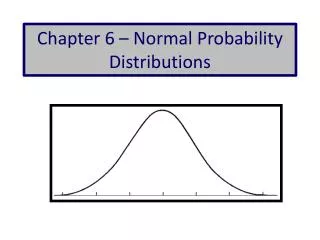
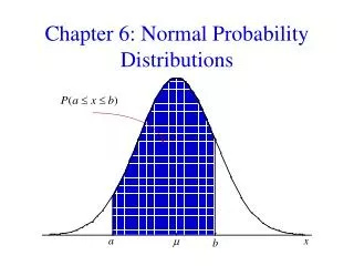
Chapter 6 Normal Probability Distributions. 6-1 Overview 6-2 The Standard Normal Distribution 6-3 Applications of Normal Distributions 6-4 Sampling Distributions and Estimators 6-5 The Central Limit Theorem 6-6 Normal as Approximation to Binomial 6-7 Assessing Normality.

E N D
Chapter 6Normal Probability Distributions 6-1 Overview 6-2 The Standard Normal Distribution 6-3 Applications of Normal Distributions 6-4 Sampling Distributions and Estimators 6-5 The Central Limit Theorem 6-6 Normal as Approximation to Binomial 6-7 Assessing Normality
Section 6-1 Overview
Overview Chapter focus is on: • Continuous random variables • Normal distributions x- )2 ( -1 e2 f(x) = 2 p Formula 6-1 Figure 6-1
Section 6-2 The Standard Normal Distribution
Key Concept • This section presents the standard normal distribution which has three properties: • It is bell-shaped. • It has a mean equal to 0. • It has a standard deviation equal to 1. • It is extremely important to develop the skill to find areas (or probabilities or relative frequencies) corresponding to various regions under the graph of the standard normal distribution.
Definition • A continuous random variable has a uniform distribution if its values spread evenly over the range of probabilities. The graph of a uniform distribution results in a rectangular shape.
Definition • A density curve is the graph of a continuous probability distribution. It must satisfy the following properties: 1. The total area under the curve must equal 1. 2. Every point on the curve must have a vertical height that is 0 or greater. (That is, the curve cannot fall below the x-axis.)
Area and Probability Because the total area under the density curve is equal to 1, there is a correspondence between area and probability.
Example A statistics professor plans classes so carefully that the lengths of her classes are uniformly distributed between 50.0 min and 52.0 min. That is, any time between 50.0 min and 52.0 min is possible, and all of the possible values are equally likely. If we randomly select one of her classes and let x be the random variable representing the length of that class, then x has a distribution that can be graphed as:
Figure 6-3 Example Kim has scheduled a job interview immediately following her statistics class. If the class runs longer than 51.5 minutes, she will be late for her job interview. Find the probability that a randomly selected class will last longer than 51.5 minutes given the uniform distribution illustrated below.
There are many different kinds of normal distributions, but they are both dependent upon two parameters… Population Mean Population Standard Deviation
Definition • The standard normal distribution is a probability distribution with mean equal to 0 and standard deviation equal to 1, and the total area under its density curve is equal to 1.
Finding Probabilities - Table A-2 • Table A-2 (Inside back cover of textbook, Formulas and Tables card, Appendix) • STATDISK • Minitab • Excel • TI-83/84
Using Table A-2 z Score Distance along horizontal scale of the standard normal distribution; refer to the leftmost column and top rowofTable A-2. Area Region under the curve; refer to the values in the body of Table A-2.
Example - Thermometers If thermometers have an average (mean) reading of 0 degrees and a standard deviation of 1 degree for freezing water, and if one thermometer is randomly selected, find the probability that, at the freezing point of water, the reading is less than 1.58 degrees.
Example - Cont P(z< 1.58) = Figure 6-6
Example - cont P (z< 1.58) = 0.9429 Figure 6-6
Example - cont P (z< 1.58) = 0.9429 The probability that the chosen thermometer will measure freezing water less than 1.58 degrees is 0.9429.
Example - cont P (z< 1.58) = 0.9429 94.29% of the thermometers have readings less than 1.58 degrees.
Example - cont If thermometers have an average (mean) reading of 0 degrees and a standard deviation of 1 degree for freezing water, and if one thermometer is randomly selected, find the probability that it reads (at the freezing point of water) above –1.23 degrees. The probability that the chosen thermometer with a reading above -1.23 degrees is 0.8907. P (z> –1.23) = 0.8907
Example - cont 89.07% of the thermometers have readings above –1.23 degrees. P (z> –1.23) = 0.8907
Athermometer is randomly selected. Find the probability that it reads (at the freezing point of water) between –2.00 and 1.50 degrees. Example - cont The probability that the chosen thermometer has a reading between – 2.00 and 1.50 degrees is 0.9104. P (z< –2.00) = 0.0228 P (z< 1.50) = 0.9332 P (–2.00 < z< 1.50) = 0.9332 –0.0228 = 0.9104
Example - Modified Athermometer is randomly selected. Find the probability that it reads (at the freezing point of water) between –2.00 and 1.50 degrees. If many thermometers are selected and tested at the freezing point of water, then 91.04% of them will read between –2.00 and 1.50 degrees. P (z< –2.00) = 0.0228 P (z< 1.50) = 0.9332 P (–2.00 < z< 1.50) = 0.9332 –0.0228 = 0.9104
Notation P(a < z < b) denotes the probability that the z score is between a and b. P(z > a) denotes the probability that the z score is greater than a. P(z < a) denotes the probability that the z score is less than a.
Finding a z Score When Given a Probability Using Table A-2 1. Draw a bell-shaped curve, draw the centerline, and identify the region under the curve that corresponds to the given probability. If that region is not a cumulative region from the left, work instead with a known region that is a cumulative region from the left. 2. Using the cumulative area from the left, locate the closest probability in the body of Table A-2 and identify the corresponding z score.
Finding z Scores When Given Probabilities Using the same thermometers as earlier, find the temperature corresponding to the 95th percentile. That is, find the temperature separating the bottom 95% from the top 5%. 5% or 0.05 (z score will be positive) Figure 6-10 Finding the 95th Percentile
Finding z Scores When Given Probabilities - cont 5% or 0.05 (z score will be positive) 1.645 Figure 6-10 Finding the 95th Percentile
Using the same thermometers, find the temperatures separating the bottom 2.5% from the top 2.5%. (One z score will be negative and the other positive) Figure 6-11 Finding the Bottom 2.5% and Upper 2.5%
Finding z Scores When Given Probabilities - cont (One z score will be negative and the other positive) Figure 6-11 Finding the Bottom 2.5% and Upper 2.5%
Finding z Scores When Given Probabilities - cont (One z score will be negative and the other positive) Figure 6-11 Finding the Bottom 2.5% and Upper 2.5%
Recap • In this section we have discussed: • Density curves. • Relationship between area and probability • Standard normal distribution. • Using Table A-2.