Download
1 / 34
340 likes | 557 Views
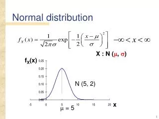
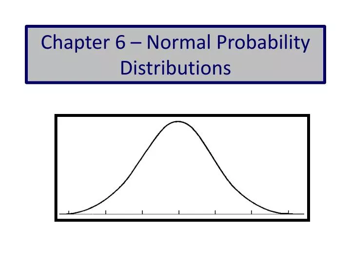
Chapter 6 – Normal Probability Distributions. Normal Distribution. If a continuous random variable has a distribution with a graph that is symmetric and bell-shaped and it satisfies the equation w e say that it has a normal distribution . ***No! We will never use this formula!.

E N D
Normal Distribution If a continuous random variable has a distribution with a graph that is symmetric and bell-shaped and it satisfies the equation we say that it has a normal distribution. ***No! We will never use this formula!
Density Curves A density curve links a probability to an area under the curve and above the x-axis. The total area under the curve is 1.
Standard Normal Distribution • Graph is bell-shaped • Mean is equal to 0 • Standard deviation is equal to 1.
z-score Table Appendix A Table A - 2 z-score are given to two decimal places Probabilities are given to four decimal places Negative z-scores Positive z-scores Numbers inside the table represent areas to the left of the z-score.
Find the Shaded Area P = 0.5871 P = 0.0047 z = 0.22 z = -2.60 P = 0.7389 P = 0.3632 z = -0.35 z = 0.64
Find the z-score P = 0.9678 P = 0.1781 z = 1.85 z = -0.92 P = 0.8588 P = 0.0134 z = 1.08 z = -2.22
Critical Values A critical value is a z-score on the borderline separating the z-scores that are likely to occur from those that are unlikely to occur. Common critical values are z = -1.96 and z = 1.96 Recall the Empirical Rule: Above 2 or below -2 were considered unusual. The notation denotes the z-score with an area of in its tail. Always rewrite to four decimal places!
Critical Values The area in the tail is 0.0700. That means the area above the positive z-score is 0.0700 and the area below the negative z-score is 0.0700. The total area under the curve is 1. 1 – 0.0700 = 0.9300
Critical Values The area in the tail is 0.1000. That means the area above the positive z-score is 0.1000 and the area below the negative z-score is 0.1000. The total area under the curve is 1. 1 – 0.1000 = 0.9000
Find the Probability The area to the left of z = 0.58 0.7190 0.2810 The area to the left of z = -0.58
Find the Probability The area to the left of z = 0.02 0.5080 0.0885 The area to the left of z = -1.35
Heights Heights Men’s heights are normally distributed with mean 68.9 in and standard deviation of 2.8 in. Women’s heights are normally distributed with mean 63.5 in and standard deviation of 2.5 in. The standard doorway height is 80 in. a. What percentage of men are too tall to fit through a standard doorway without bending, and what percentage of women are too tall to fit through a standard doorway without bending?
Heights Women’s heights are normally distributed with mean 63.5 in and standard deviation of 2.5 in. The standard doorway height is 80 in. a. What percentage of women are too tall to fit through a standard doorway without bending?
Heights If a statistician designs a house so that all of the doorways have heights that are sufficient for all men except the tallest 5%, what doorway height would be used?
Heart Rates Suppose that heart rates are normally distributed with a mean of 61.4 beats per minute and a standard deviation of 3.7 beats per minute. a. If one person is selected randomly, find the probability that their heart rate is less than 62 beats per minute
Heart Rates Suppose that heart rates are normally distributed with a mean of 61.4 beats per minute and a standard deviation of 3.7 beats per minute. b. What is the probability that a person has a heart rate greater than 65 beats per minute?
Heart Rates Suppose that heart rates are normally distributed with a mean of 61.4 beats per minute and a standard deviation of 3.7 beats per minute. c. What is the probability that a person has a heart rate between 57 and 62 beats per minute?
Heart Rates Suppose that heart rates are normally distributed with a mean of 61.4 beats per minute and a standard deviation of 3.7 beats per minute. d. If 50 people are randomly selected, find the probability that they have a mean heart rate less than 62 beats per minute. (Use the Central Limit Theorem)
Law of Large Numbers Draw observations at random from any population with finite mean . As we increase the number of observations, the mean of the observed values , gets closer to the mean of the population. As we increase the sample size n, the sample mean gets closer to the population mean.
Estimators We will use sample statistics to estimate population parameters. Some sample statistics that we might use to estimate population parameters:
Estimators An estimator is unbiased if it targets the population parameter. An estimator is biased if it systematically under estimates or over estimates the population parameter. Since the bias associated with the sample standard deviation is very small, we WILL still use it to estimate the population standard deviation.
Sampling Distributions The population distribution is the distribution of the values of the variable among all the individuals of a population. The sampling distribution of a statistic is a theoretical distribution of values taken by the statistic in all possible samples of the same size from the same population. A population distribution shows how the value of an individual varies in a population. A sampling distribution shows how the value of a statistic varies from all possible samples of a certain size.
Sampling Distribution of sampling distribution of the mean The mean of the sampling distribution or The mean of the means
Sampling Distribution of An ice cream company was in business for only three days. Here are the numbers of phone calls received on each of those days: 12, 10, 5. Assume that samples of size 2 are randomly selected with replacement from this population of three values. a. List the different population samples and find the mean of each of them.
Sampling Distribution of b. Identify the probability of each sample. c. Calculate the mean of the sampling distribution.
Sampling Distribution of d. Is the mean from the sampling distribution from part (c) the same as the mean of the population of the three listed values? If so, are those means always equal? Since the mean is an unbiased estimator, it will target the population mean. Yes, the mean of the sampling distribution will always be the same as the mean of the population.
Notation Notation for the sampling distribution of : If all possible random samples of size nare selected from a population with mean and standard deviation , the mean of the sample means is denoted by , and Also the standard deviation of the sample means is denoted by , and is called the standard error of the mean.
Central Limit Theorem The Central Limit Theorem allows us to use the Normal probability calculations to answer questions about sample means from many observations even when the population distribution is NOT normal. (For strongly skewed distributions, n > 30 is a good rule of thumb) • As the sample size increase • Standard error decreases • the z score gets larger
Heart Rates Suppose that heart rates are normally distributed with a mean of 61.4 beats per minute and a standard deviation of 3.7 beats per minute. d. If 50 people are randomly selected, find the probability that they have a mean heart rate less than 62 beats per minute. (Use the Central Limit Theorem)
Heart Rates Suppose that heart rates are normally distributed with a mean of 61.4 beats per minute and a standard deviation of 3.7 beats per minute. e. If 100people are randomly selected, find the probability that they have a mean heart rate less than 62 beats per minute. (Use the Central Limit Theorem)