Download
1 / 46
580 likes | 810 Views
Normal Probability Distributions. Elementary Statistics Larson Farber. Chapter 5. N. Section 5.1. Introduction to Normal Distributions. Properties of a Normal Distribution. x. The mean, median, and mode are equal. Bell shaped and is symmetric about the mean.

E N D
Normal Probability Distributions Elementary Statistics Larson Farber Chapter 5 N
Section 5.1 Introduction to Normal Distributions
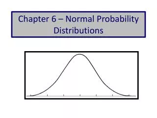
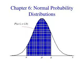
Properties of a Normal Distribution x • The mean, median, and mode are equal • Bell shaped and is symmetric about the mean • The total area that lies under the curve is one or 100%
Properties of a Normal Distribution Inflection point Inflection point x • As the curve extends farther and farther away from the • mean, it gets closer and closer to the x- axis but never touches it. • The points at which the curvature changes are called inflection points. The graph curves downward between the inflection points and curves upward past the inflection points to the left and to the right
Means and Standard Deviations 10 11 12 13 14 15 16 17 18 19 20 9 10 11 12 13 14 15 16 17 18 19 20 21 22 Curves with different means, same standard deviation Curves with different means different standard deviations
Empirical Rule About 68% of the area lies within 1 standard deviation of the mean 68% About 95% of the area lies within 2 standard deviations About 99.7% of the area lies within 3 standard deviations of the mean
Determining Intervals x 3 2 1 0 1 2 3 3.3 3.6 3.9 4.2 4.5 4.8 5.1 An instruction manual claims that the assembly time for a product is normally distributed with a mean of 4.2 hours and standard deviation 0.3 hours. Determine the interval in which 95% of the assembly times fall. 95% of the data will fall within 2 standard deviations of the mean. 4.2 - 2 (0.3) = 3.6 and 4.2 +2 (0.3) = 4.8. 95% of the assembly times will be between 3.6 and 4.8 hrs.
Section 5.2 The Standard Normal Distribution
The Standard Score (a) (b) (c) The standard score, or z-score, represents the number of standard deviations a random variable x falls from the mean. The test scores for a civil service exam are normally distributed with a mean of 152 and standard deviation of 7. Find the standard z-score for a person with a score of: (a) 161 (b) 148 (c) 152
The Standard Normal Distribution 4 3 2 1 0 1 2 3 4 The standard normal distribution has a mean of 0 and a standard deviation of 1. Using z- scores any normal distribution can be transformed into the standard normal distribution. z
Cumulative Areas z -3 -2 -1 0 1 2 3 The total area under the curve is one. • The cumulative area is close to 0 for z-scores close to -3.49. • The cumulative area for z = 0 is 0.5000 • The cumulative area is close to 1 for z scores close to 3.49.
Cumulative Areas 0.1056 z -3 -2 -1 0 1 2 3 Find the cumulative area for a z-score of -1.25. Read down the z column on the left to z = -1.2 and across to the column under .05. The value in the cell is0.1056, the cumulative area. The probability that z is at most -1.25 is 0.1056. P ( z -1.25) = 0.1056
Finding Probabilities z -3 -2 -1 0 1 2 3 To find the probability that z is less than a given value, read the cumulative area in the table corresponding to that z-score. Find P( z < -1.45) Read down the z-column to -1.4 and across to .05. The cumulative area is 0.0735. P ( z < -1.45) = 0.0735
Finding Probabilities 0.1075 Required area 0.8925 z -3 -2 -1 0 1 2 3 To find the probability that z is greater than a given value, subtract the cumulative area in the table from 1. Find P( z > -1.24) The cumulative area (area to the left) is 0.1075. So the area to the right is 1 - 0.1075 =0.8925. P( z > -1.24) = 0.8925
Finding Probabilities z -3 -2 -1 0 1 2 3 To find the probability z is between two given values, find the cumulative areas for each and subtract the smaller area from the larger. Find P( -1.25 < z < 1.17) 2. P(z < -1.25) =0.1056 1. P(z < 1.17) = 0.8790 3. P( -1.25 < z < 1.17) = 0.8790 - 0.1056 = 0.7734
Summary To find the probability that z is less than a given value, read the corresponding cumulative area. To find the probability is greater than a given value, subtract the cumulative area in the table from 1. z z z To find the probability z is between two given values, find the cumulative areas for each and subtract the smaller area from the larger. -3 -1 0 -1 0 1 2 3 -2 -3 -2 -1 0 1 2 3 -3 -2 1 2 3
Section 5.3 Normal Distributions Finding Probabilities
Probabilities and Normal Distributions 100 115 If a random variable, x is normally distributed, theprobabilitythat x will fall within an interval is equal to the area under the curve in the interval. IQ scores are normally distributed with a mean of 100 and standard deviation of 15. Find the probability that a person selected at random will have an IQ score less than 115. To find the area in this interval, first find the standard score equivalent to x = 115.
Probabilities and Normal Distributions Normal Distribution Find P(x < 115) SAME 100 115 SAME 1 0 Standard Normal Distribution Find P(z < 1) P( z < 1) = 0.8413, so P( x <115) = 0.8413
Application Normal Distribution Monthly utility bills in a certain city are normally distributed with a mean of $100 and a standard deviation of $12. A utility bill is randomly selected. Find the probability it is between $80 and $115. P(80 < x < 115) P(-1.67 < z < 1.25) 0.8944 - 0.0475 = 0.8469 The probability a utility bill is between $80 and $115 is 0.8469.
Section 5.4 Normal Distributions Finding Values
From Areas to z-scores 4 3 2 1 0 1 2 3 4 Find the z-score corresponding to a cumulative area of 0.9803. 0.9803 0.9803 z Locate 0.9803 in the area portion of the table. Read the values at the beginning of the corresponding row and at the top of the column. The z-score is 2.06. z = 2.06 corresponds roughly to the 98th percentile.
Finding z-scores From Areas z 0 Find the z-score corresponding to the 90th percentile. .90 The closest table area is .8997. The row heading is 1.2 and column heading .08. This corresponds to z = 1.28. A z-score of 1.28 corresponds to the 90th percentile.
Finding z-scores From Areas .40 .60 z z 0 Find the z-score with an area of .60 falling to its right. With .60 to the right, cumulative area is .40. The closest area is .4013. The row heading is –0.2 and column heading is .05. The z-score is –0.25. A z-score of –0.25 has an area of .60 to its right. It also corresponds to the 40th percentile
Finding z-scores From Areas -z z 0 Find the z-score such that 45% of the area under the curve falls between –z and z. .275 .275 .45 The area remaining in the tails is .55. Half this area is in each tail, so since .55/2 =.275 is the cumulative area for the negative z value and .275 + .45 = .725 is the cumulative area for the positive z. The closest table area is .2743 and the z-score is –0.60. The positive z score is 0.60.
From z-Scores to Raw Scores To find the data value, x when given a standard score, z: The test scores for a civil service exam are normally distributed with a mean of 152 and standard deviation of 7. Find the test score for a person with a standard score of (a) 2.33 (b) -1.75 (c) 0 (a) x = 152 + (2.33)(7) = 168.31 (b) x = 152 + ( -1.75)(7) = 139.75 (c) x = 152 + (0)(7) = 152
Finding Percentiles or Cut-off values 90% 10% To find the corresponding x-value, use Monthly utility bills in a certain city are normally distributed with a mean of $100 and a standard deviation of $12. What is the smallest utility bill that can be in the top 10% of the bills? z Find the cumulative area in the table that is closest to 0.9000 (the 90th percentile.) The area 0.8997 corresponds to a z-score of 1.28. x = 100 + 1.28(12) = 115.36. $115.36 is the smallest value for the top 10%.
Section 5.5 The Central Limit Theorem
Sampling Distributions The sampling distribution consists of the values of the sample means, A sampling distribution is the probability distribution of a sample statistic that is formed when samples of size n are repeatedly taken from a population. If the sample statistic is the sample mean, then the distribution is the sampling distribution of sample means. Sample Sample Sample Sample Sample Sample
The Central Limit Theorem If a sample n 30 is taken from a population withany type distribution that has a mean = and standard deviation = x and standard deviation with a mean the sample means will have a normal distribution
The Central Limit Theorem If a sample of any size is taken from a population witha normal distribution with mean = and standard deviation= x the distribution of means of sample size n , will be normal with a mean standard deviation
Application The mean height of American men (ages 20-29) is inches. Random samples of 60 such men are selected. Find the mean and standard deviation (standard error) of the sampling distribution. mean 69.2 Standard deviation Distribution of means of sample size 60 , will be normal.
Interpreting the Central Limit Theorem Since n > 30 the sampling distribution of will be normal standard deviation The mean height of American men (ages 20-29) is = 69.2”. If a random sample of 60 men in this age group is selected, what is the probability the mean height for the sample is greater than 70”? Assume the standard deviation is 2.9”. mean Find the z-score for a sample mean of 70:
Interpreting the Central Limit Theorem P ( > 70) 2.14 Interpreting the Central Limit Theorem = P (z > 2.14) = 1 - 0.9838 = 0.0162 z There is a 0.0162 probability that a sample of 60 men will have a mean height greater than 70”.
Application Central Limit Theorem Since n > 30 the sampling distribution of will be normal mean During a certain week the mean price of gasoline in California was $1.164 per gallon. What is the probability that the mean price for the sample of 38 gas stations in California is between $1.169 and $1.179? Assume the standard deviation = $0.049. standard deviation Calculate the standard z-score for sample values of $1.169 and $1.179.
Application Central Limit Theorem z .63 1.90 P( 0.63 < z < 1.90) = 0.9713 - 0.7357 = 0.2356 The probability is 0.2356 that the mean for the sample is between $1.169 and $1.179.
Section 5.6 Normal Approximation to the Binomial
Binomial Distribution Characteristics • There are a fixed number of independent trials. (n) • Each trial has 2 outcomes, Success or Failure. • The probability of success on a single trial is p and the probability of failure is q. p + q = 1 • We can find the probability of exactly x successes out of n trials. Where x = 0 or 1 or 2 … n. • x is a discrete random variable representing a count of the number of successes in n trials.
Application If np 5 and nq 5, the binomial random variable x is approximately normally distributed with mean and 34% of Americans have type A+ blood. If 500 Americans are sampled at random, what is the probability at least 300 have type A+ blood? Using techniques of chapter 4 you could calculate the probability that exactly 300, exactly 301…exactly 500 Americans have A+ blood type and add the probabilities. Or…you could use the normal curve probabilities to approximate the binomial probabilities.
Why do we require np 5 and nq 5? 0 1 2 3 4 5 4 0 10 20 30 40 50 n = 5 p = 0.25, q = .75 np =1.25 nq = 3.75 n = 20 p = 0.25 np = 5 nq = 15 4 n = 50 p = 0.25 np = 12.5 nq = 37.5
Binomial Probabilities 0.111 0.089 0.065 14 15 16 The binomial distribution is discrete with a probability histogram graph. Theprobability that a specific value ofxwill occur is equal to the areaof the rectangle with midpoint at x. If n = 50 and p = 0.25 find P (14 x 16) Add the areas of the rectangles with midpoints at x = 14, x = 15, x = 16. 0.111 + 0.089 + 0.065 = 0.265 P (14 x 16) = 0.265
Correction for Continuity 14 15 16 Use the normal approximation to the binomial to find P(14 x 16) if n = 50 and p = 0.25 Check that np= 12.5 5 and nq= 37.5 5. Values for the binomial random variable x are 14, 15 and 16.
Correction for Continuity 14 15 16 Use the normal approximation to the binomial to find P(14 x 16) if n = 50 and p = 0.25 Check that np= 12.5 5 and nq= 37.5 5. The interval of values under the normal curve is 13.5 x 16.5. To ensure the boundaries of each rectangle are included in the interval, subtract 0.5 from a left-hand boundary and add 0.5 to a right-hand boundary.
Normal Approximation to the Binomial Use the normal approximation to the binomial to find P(14 x 16) if n = 50 and p = 0.25 Find the mean and standard deviation using binomial distribution formulas. Adjust the endpoints to correct for continuity P(13.5 x 16.5) Convert each endpoint to a standard score P(0.33 z 1.31) = 0.9049 - 0.6293 = 0.2756
Application A survey of Internet users found that 75% favored government regulations on “junk” e-mail. If 200 Internet users are randomly selected, find the probability that fewer than 140 are in favor of government regulation. Since np = 150 5 and nq = 50 5 use the normal approximation to the binomial. The binomial phrase of “fewer than 140” means 0, 1, 2, 3…139. Use the correction for continuity to translate to the continuous variable in the interval (- , 139.5). Find P( x < 139.5 )
Application A survey of Internet users found that 75% favored government regulations on “junk” e-mail. If 200 Internet users are randomly selected, find the probability that fewer than 140 are in favor of government regulation. Use the correction for continuity P(x < 139.5) P( z < -1.71) = 0.0436 The probability that fewer than 140 are in favor of government regulation is approximately 0.0436