Download
1 / 22
220 likes | 229 Views
The Climate Change – Urban Pollution Relationship. Effects of climate change on air quality Effects of aerosols on regional climate. Smog over Pittsburgh, ranked #1 city for particulate pollution in 2008 by ALA. Loretta J. Mickley, Harvard University

E N D
The Climate Change – Urban Pollution Relationship • Effects of climate change on air quality • Effects of aerosols on regional climate Smog over Pittsburgh, ranked #1 city for particulate pollution in 2008 by ALA Loretta J. Mickley, Harvard University also Shiliang Wu, Jennifer Logan, Dominick Spracklen, Amos Tai, Rynda Hudman, Daniel Jacob, Moeko Yoshitomi, Eric Leibensperger, Havala Pye Funding for this work: NASA, EPA, EPRI
Millions of people already live in areas of high pollution. Number of people living in areas that exceed the national ambient air quality standards (NAAQS) in 2006. 0.08 ppm Calculated with old 0.08 ppm standard. New standard of 0.075 ppm will push more areas into non-attainment. 65 mg/m3 EPA’s Technical Support Document for the proposed finding on CO2 as a pollutant. Cites the threat of climate change to air quality.
O2 hn Chemistry of tropospheric ozone: oxidation of CO, VOCs, and methane in the presence of NOx O3 STRATOSPHERE 8-18 km TROPOSPHERE Stagnation promotes ozone production hn NO2 NO O3 hn, H2O OH HO2 H2O2 Deposition CO, VOC Nitrogen oxide radicals;NOx = NO + NO2 combustion, soil, lightning Methane wetlands, livestock, natural gas Nonmethane volatile organic compounds (VOCs) vegetation, combustion, industry CO (carbon monoxide) combustion, VOC oxidation Tropospheric ozone precursors
Number of summer days with ozone exceedances, mean over sites in Northeast Northeast Probability of ozone exceedance vs. daily max. temperature • Curves include effects of • Biogenic emissions • Stagnation • Clear skies Probability Days 1988, hottest on record Southeast Los Angeles Temperature (K) Weather plays a large role in ozone air quality. The total derivative d[O3]/dT is the sum of partial derivatives (dO3/dxi)(dxi/dT). x = ensemble of ozone forcing variables that are temperature-related. Lin et al., 2001
Cyclones crossing southern Canada affect ozone air quality in Eastern US. cold front L EPA ozone levels • Stalled high pressure system associated with: • increased biogenic emissions • clear skies • weak winds • high temperatures. cold front L 3 days later Cold front pushes smog poleward and aloft on a warm conveyor belt. Hazardous levels of ozone
cyclones 0.14 a-1 NE ozone episodes 0.16 a-1 Decline in mid-latitude cyclone number over mid-latitudes leads to more persistent stagnation episodes, more ozone. 1950-2006 trend in JJA cyclones in S. Canada Trend in cyclones appears due in part to weakened meridional temperature gradients, reduction of baroclinicity over midlatitudes. 1980-2006 trends Trend in emissions and trend in cyclones have competing effects on surface ozone. If cyclone frequency had remained constant, we calculate zero episodes over Northeast. Mickley et al., 2004; Leibensperger et al., 2008
. . . . . . Particulate matter (PM, aerosols) sources and processes ultra-fine (<0.01 mm) fine (0.01-1 mm) cloud (1-100 mm) precursor gases oxidation nucleation cycling coagulation H2SO4 SO2 condensation RCO… VOCs coarse (1-10 mm) scavenging NOx HNO3 wildfires NH3 carbonaceous combustion particles combustion biosphere volcanoes agriculture biosphere soil dust sea salt
Observed correlations of total PM2.5 with meteorology • Precipitation • Stagnation • Temperature • Positive correlation with temperature occurs due to: • Increased oxidation of SO2 • Greater biogenic emissions Precipitation Stagnation Results from EPA AQS database: 1000+ sites sampled every 1-6 days from 1998 to 2007. Observed correlations provide means to test model simulations. E.g., observed sulfate response to temperature is ~ +0.08 μg m-3/K, 4x greater than Dawson et al. 2007 model. Temperature Tai et al., ms.
2000-2050 decrease in cyclone frequency leads to increased stagnation. 2050s CO tracer Northeast, Jul-Aug 1990s AIR QUALITY What do models project for future air quality? We have developed GCAP (Global Change and Air Pollution). GISS GCM Physics of the atmosphere Qflux ocean or specified SSTs GEOS-Chem Emissions Chemical scheme Deposition met fields met fields chemistry fields met fields Regional chemistry model Regional climate model Chemistry model driven by GCM meteorology to study influence of climate on air quality. Mickley et al., 2004
2000-2050 climate change increases JJA surface ozone: 1-5 ppb on average across US, 5-10 ppb during heat waves in Midwest Max. 8-hr-avg ozone Effect of climate change alone 2000s conditions 2050s climate 2050s emissions 2050s climate & emis Increase of summer max-8h-avg ozone 99th percentile Cumulative probability (%) Midwest Daily max 8h-avg ozone averaged in JJA (ppb) We define the climate change penalty as the effort required to meet air quality standards under future climate change. Wu et al., 2007
Change in annual mean surface inorganic aerosol from 2000-2050 climate change (no change in emissions) Increase in Northeast due to increased temperature and accelerated oxidation rates Decrease in Southeast due mainly to increased precipitation. Calculation of future aerosol levels is challenging because of uncertainty in future rainfall over mid-latitudes. Also, mix of aerosol species is expected to change, so sensitivity to climate will also change. Present-day annual average Pye et al., 2009 sulfate nitrate ammonium
May-Oct area burned in Pacific Northwest observations 0.5 R2=52% model Area burned / 106 Ha 0.25 1980 1990 1990 2000 Perturbation due to climate change only Projected increase in wildfires could affect air quality in the US. We predict future wildfires using observed relationships between meteorology and area burned for different ecosystems. 2000-2050 changes in fire season surface ozone. Spracklen et al., 2009 Hudman et al, ms.
Present-day radiative forcing due to aerosols over the eastern US is comparable in magnitude, but opposite in sign, to global forcing due to CO2. Globally averaged radiative forcing due to CO2 is +1.7 Wm-2. warming Over the eastern US, radiative forcing due to sulfate aerosols is -2 Wm-2. cooling IPCC, 2007; Liao et al. , 2004
Is the climate response to changing aerosols collocated with regions of radiative forcing? Recent US Climate Change report says NO: Trends in short-lived species (such as aerosols) affect global, but not regional, climate. “Regional emissions control strategies for short-lived pollutants will . . . have global impacts on climate.” – U.S. Climate Change Science Program, Synthesis and Assessment Product 3.2 Harvard’s work to date says YES: Removal of the aerosol burden over the eastern US will lead to regional warming, in a way that the US Climate Change report would not have recognized. Calculated present-day aerosol optical depths
What is the influence of changing aerosol on regional climate? In pilot study, we zero out aerosol optical depths over US. GISS GCM For pilot study, 2 scenarios were simulated: Control: aerosol optical depths fixed at 1990s levels. Sensitivity: U.S. aerosol optical depths set to zero (providing a radiative forcing of about +2 W m-2 locally over the US); elsewhere, same as in control simulation. Each scenario includes an ensemble of 3 simulations.
Removal of anthropogenic aerosols over US leads to a 0.5-1o C warming in annual mean surface temperature. Additional warming due to zeroing of aerosols over the US. Warming due to 2010-2025 trend in greenhouse gases. Annual mean surface temperature change in Control. Mean 2010-2025 temperature difference: No-US-aerosol case – Control White areas signify no significant difference. Results from an ensemble of 3 for each case. Mickley et al., ms.
No-US-aerosols case Temperature (oC) Control, with US aerosols The regional surface temperature response to aerosol removal appears to persist for many decades in the model. Annual mean temperature trends over Eastern US Temperature response is initially strongest in winter. Summertime temperature response kicks in around 2030. Mickley et al., ms
Implications for policymakers • Policymakers need to consider “climate change penalty,” i.e., the additional emission controls necessary to meet a given air quality target. • Efforts to clear the air of anthropogenic aerosol over the US may exacerbate regional warming. Directions for future research Understand causes in interannual variability of air quality. Investigate model sensitivity of pollutants to meteorology, and compare to observations. Understand chemistry of biogenic species, e.g. isoprene Improve emission inventories for recent past/future, especially for NH3, black carbon, organic carbon, mercury Improve global and regional models of mercury Understand secondary organic aerosols: sources, chemistry. For cities: improve modeling of fine scale features, investigate how best to downscale meteorology from global climate models, test effects of land use change. Understand aerosol-cloud interactions, characterize aerosol composition
Ozone exceedances in eastern US correlate with frequency of cyclone passage through southern Canada/Great Lakes region. Correlation between cyclone number in red and green boxes and US ozone exceedances over 27-year record, JJA Storm tracks for 3 years (NCEP, summer 1979-1981) Storm tracks calculated with cyclone tracker tool, applies cyclone criteria to observations or model output. Leibensperger et al., 2008
Perturbation due to climate change only Projected increase in wildfires could affect air quality in the US. 2000-2050 change in JJA surface organic aerosol due to increased wildfires We have developed a fire prediction tool based on observed relationships between meteorology and area burned. Applying these relationships to GCM meteorology, we predict area burned and future emissions of wildfire pollutants. mg m-3 Changes in JJA surface ozone concentrations Spracklen et al., 2009 Hudman et al, ms.
We define the climate change penalty as the effort required to meet air quality goals in the future atmosphere. 40% cut in NOx + 2050s climate present-day NOx emissions + climate } climate change penalty 40% cut in NOx + present-day climate 50% cut in NOx + 2050s climate 2000–2050 climate change implies an additional 25% effort in NOx emission controls to achieve the same ozone air quality. Midwest surface ozone Wu et al., 2007