Download
1 / 42
490 likes | 779 Views
Fluke 190-204 Oscilloscope. 4 Isolated Channels 200 Mhz Bandwidth CAT III 1000 CAT IV 600 Rated 2.5 GS/s sample rate Connect-and-View™ IP-51 Rated. Z axis, Frequency (Hertz). Y axis, Amplitude (Volts, dB). Volts. time. X axis, time (Seconds). Oscilloscopes.

E N D
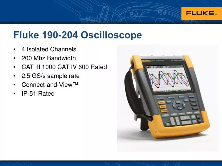
Fluke 190-204 Oscilloscope • 4 Isolated Channels • 200 Mhz Bandwidth • CAT III 1000 CAT IV 600 Rated • 2.5 GS/s sample rate • Connect-and-View™ • IP-51 Rated
Z axis, Frequency (Hertz) Y axis, Amplitude (Volts, dB) Volts time X axis, time (Seconds) Oscilloscopes • A multimeter precisely measures a signals amplitude • An osciloscope displays a signal amplitude change over time • A spectrum analyzer displays a signal power level (amplitude) with respect to frequency • Electrical Signals are measured in three domains 110.56 Vac dB Frequency
Amplitude in Volts Time in Seconds What is a multimeter? • A Multimeter accurately displays discreet Volts, Ohms and Amp measurements. • A typical multimeter uses an integrating ADC to convert an unknown voltage • An integrating capacitor is charged for a precise time span, then discharged. • The discharge time is proportionate to the unknown signal charging the integrator. • The longer the integration time, the higher the resolution, therefore more accurate the measurement becomes. Accuracies as low as 10’s of parts per million (0.001 %) can be achieved
Amplitude in Volts Time in Seconds What is an Oscilloscope? • An Oscilloscope graphically plots signals over time • The oscilloscope using high speed A to D conversion, samples the unknown input as fast as possible then graphically plots the unknown samples over time “A picture is worth a thousand words!”
DMM or Oscilloscope? • A multimeter, presents a single precise measured value • An oscilloscope presents a graphical representation of a signal change over time. • To obtain precise measurements, the typical DMM converts the unknown input at a rate of 5 or 10 times per second • To accurately represent a signal change over time, an oscilloscope can sample the unknown input up to 2.5 billion times per second (or faster)
Micro Processor Lf Ch A 2.5 GSa/s A/D Hf Memory Optional Ch Isolation Digital Storage Oscilloscope • Input Coupling • AC or DC • Amplitude Control • Attenuation • Amplification • Channel Isolation • Up to 1000 Volt isolation • Available on some scopes • A to D Conversion • Real time • Up to 2.5 GSa/s • Triggering • Edge • Edge Delay • Pulse Width • N-Cycle • System Control • Sample Storage • Measure functions • Graphics processing • User interface
Input Coupling • Input coupling determines what is passed on to the signal conditioning circuit • AC, Passes AC component only • DC, Passes both AC and DC components of the signal Applied Input Resultant Output DC Coupling Gnd Ref AC & DC Signal Components AC Coupling Gnd Ref Gnd Ref AC Signal Component, DC is blocked by capacitor
Display Amplitude Control • Controls the vertical span of the displayed signal, adjusted in volts per vertical display division • mV increases sensitivity • V decreases sensitivity Vertical Sensitivity (V/Div) Amplitude display range Gnd Ref mV Pressing mV increases vertical sensitivity Gnd Ref V Gnd Ref Pressing V deceases vertical sensitivity
Gnd Ref Analog to Digital Conversion • The unknown signal is applied to the analog to digital converter (A/D). • The A/D process divides the signal into segments at specified time intervals. • At each time interval the voltage of the signal is determined and stored into memory Storage Memory 1 2 3 4 5 6 . . . . . . . 1000 A to D Conversion Gnd Ref mS/Div S/Div Horizontal Time base (s/Div) Sampling clock interval time Horizontal resolution
Sample Rate & Memory • A digital storage oscilloscope contains a fixed amount of memory points • The more memory, the higher the cost and the longer it takes to fill up over a complete acquisition cycle • The fewer memory points the lower the resolution, the displayed signal time span and frequency bandwidth • The sample rate will increase or decrease relative to the amount of memory and maximum sample rate • It will automatically adjust the sample rate from its maximum at the fastest time base setting (nano seconds/div) to a slower sample rate at the slower time base settings (example, milli seconds/div) Cost Memory Depth time gS Sample Rate S ns Min Time base
Digital Oscilloscope Aliasing • If the acquisition rate is much slower than the frequency of the measured signal Aliasing can occur • Aliasing displays incorrect signals Actual Signal Signal observed when Aliasing occurs
A/D – Glitch Detection • Glitch Detect • At slow time base settings/ sampling intervals the A/D can miss glitches • Over sampling captures min and max sample points, preventing aliasing and displaying glitches Digitized Signal Display Pixels Actual Signal Displayed Max Sample • Over Sampling Glitch Detect • The Min & Max samples displayed in each column Displayed Min Sample
Oscilloscope Bandwidth • Bandwidth, determines the highest signal frequency the oscilloscope can accurately reproduce • The maximum frequency is usually determined by measuring the point at which the amplitude decreases as frequency increases by no more than -3 db’s (30% change) • Bandwidth is also dependent on sampling rate Test Signal Volume Frequency 1 Frequency 2 Frequency 3 Perceived Volume
Triggering • Triggering, synchronizes the waveform display process every time the waveform is refreshed or displayed. Composite image of “Un-Triggered” scope 1 Acquisition cycles 4 2 Triggered, resulting in stable display 3 T
Triggering Techniques • Oscilloscopes use several techniques to trigger on unknown signals • Edge, a specific voltage level set relative to either a rising or falling edge. • Pulse Width, specifies both a specific voltage level relative to an edge, plus a time interval between the rise and falling edges (or visa versa). • Automatic Connect&View: • As implied, connect then view, as simple as that! • Eliminates need to continuously adjust the scope vertical sensitivity, horizontal time and trigger settings V level time V level Trigger V/Div Time/Div
Ref A Ref B Oscilloscope Isolation • The ScopeMeter input connectors are insulated to prevent against exposure to electrical voltages • The input power adapter is isolated from earth ground, allowing for floating measurements • A typical bench oscilloscope uses metal BNC connectors and metal chassis components, potentially exposing the user to hazardous voltages. • To protect against electric shock the bench oscilloscope is connected directly to earth ground via wall outlet. AC to DC Power Adapter, specially designed to meet CAT II 1000V/ CAT III 600V Safety rating Isolated adapter DC Out
CH B Signal Input CH A Signal Input Common reference tied to earth ground CH A Reference Input CH B Reference Input CH B Signal Input CH A Signal Input CAT II 1000 V/ CAT III 600V Isolation Channel Isolation • Bench oscilloscope with exposed metal BNC connectors and common input references, for safety reasons are tied to earth ground • Fluke 190 series portable oscilloscope with insulated BNC input connectors isolated from earth ground with isolated input references The Fluke ScopeMeter test tools provide a safe means to measure floating differential voltages
Using the 190-204 Oscilloscope • Input Connections • BNC Connectors are 300V CAT IV • Fluke 10:1 Probes provide 1000V CAT III600V CAT IV
Using the 190-204 Oscilloscope • Resetting the 190-204 to factory settings
Using the 190-204 Oscilloscope • Hiding Labels and Key Illumination meaning
Using the 190-204 Oscilloscope • Probe Settings
Using the 190-204 Oscilloscope • Selecting Input Channels
Using the 190-204 Oscilloscope • Connect-and-View™
Using the 190-204 Oscilloscope • Automatic Measurements
Using the 190-204 Oscilloscope • Average, Persistance, and Glitch Capture
Using the 190-204 Oscilloscope • Displaying Glitches and suppressing High Frequency Noise
Using the 190-204 Oscilloscope • Acquisition Rate
Using the 190-204 Oscilloscope • AC/DC Coupling
Using the 190-204 Oscilloscope • Bandwidth and Noisy Waveforms
Using the 190-204 Oscilloscope • Mathematics (FFT)
Using the 190-204 Oscilloscope • Reference Trace
Using the 190-204 Oscilloscope • Meter Mode
Using the 190-204 Oscilloscope • Trend Plot Meter
Using the 190-204 Oscilloscope • ZOOM Button
Using the 190-204 Oscilloscope • CURSOR Button
Using the 190-204 Oscilloscope • Record Waveforms in Deep Memory
Using the 190-204 Oscilloscope • Scope Record in Single SweepMode
Using the 190-204 Oscilloscope • REPLAY Button
Using the 190-204 Oscilloscope • Trigger Level
Using the 190-204 Oscilloscope • Saving and Recalling
Using the 190-204 Oscilloscope • FlukeView Scope Software Demonstration
Conclusion • Questions?