Download
1 / 29
560 likes | 971 Views
For Electrical Engineering and Physics Undergraduate Students. Oscilloscope Fundamentals. Agenda. What is an oscilloscope? Probing basics (low-frequency model) Making voltage and timing measurements Properly scaling waveforms on-screen Understanding oscilloscope triggering

E N D
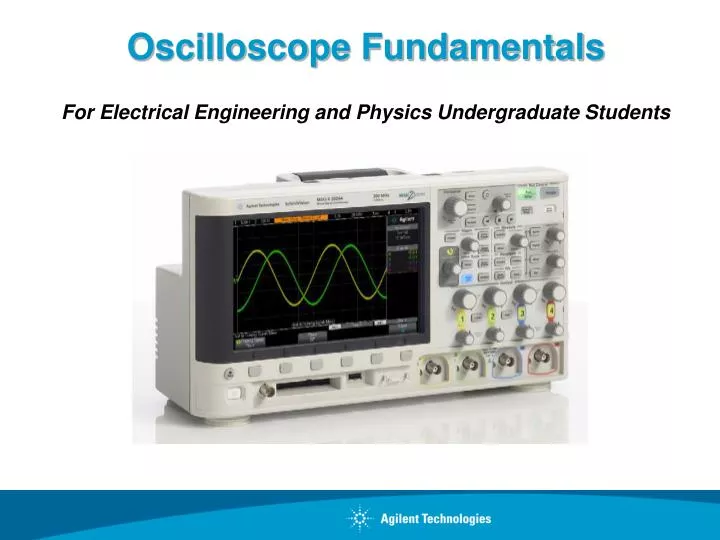
For Electrical Engineering and Physics Undergraduate Students Oscilloscope Fundamentals
Agenda • What is an oscilloscope? • Probing basics (low-frequency model) • Making voltage and timing measurements • Properly scaling waveforms on-screen • Understanding oscilloscope triggering • Oscilloscope theory of operation and performance specifications • Probing revisited (dynamic/AC model and affects of loading) • Using the DSOXEDK Lab Guide and Tutorial • Additional technical resources
What is an oscilloscope? • Oscilloscopes convert electrical input signals into a visible trace on a screen - i.e. they convert electricity into light. • Oscilloscopes dynamically graph time-varying electrical signals in two dimensions (typically voltage vs. time). • Oscilloscopes are used by engineers and technicians to test, verify, and debug electronic designs. • Oscilloscopes will be the primary instrument that you will use in your EE/Physics labs to test assigned experiments. os·cil·lo·scope (ə-sĭl'ə-skōp')
Terms of Endearment (what they are called) • Scope – Most commonly used terminology • DSO – Digital Storage Oscilloscope • Digital Scope • Digitizing Scope • Analog Scope – Older technology oscilloscope, but still around today. • CRO – Cathode Ray Oscilloscope (pronounced “crow”). Even though most scopes no longer utilize cathode ray tubes to display waveforms, Aussies and Kiwis still affectionately refer to them as their CROs. • O-Scope • MSO – Mixed Signal Oscilloscope (includes logic analyzer channels of acquisition)
Probing Basics • Probes are used to transfer the signal from the device-under-test to the oscilloscope’s BNC inputs. • There are many different kinds of probes used for different and special purposes (high frequency applications, high voltage applications, current, etc.). • The most common type of probe used is called a “Passive 10:1 Voltage Divider Probe”.
Passive 10:1 Voltage Divider Probe • Passive: Includes no active elements such as transistors or amplifiers. • 10-to-1: Reduces the amplitude of the signal delivered to the scope’s BNC input by a factor of 10. Also increases input impedance by 10X. • Note: All measurements must be performed relative to ground! Passive 10:1 Probe Model
Low-frequency/DC Model • Low-frequency/DC Model: Simplifies to a 9-MΩ resistor in series with the scope’s 1-MΩ input termination. • Probe Attenuation Factor: • Some scopes such as Agilent’s 3000 X-Series automatically detect 10:1 probes and adjust all vertical settings and voltage measurements relative to the probe tip. • Some scopes such as Agilent’s 2000 X-Series require manual entry of a 10:1 probe attenuation factor. • Dynamic/AC Model: Covered later and during Lab #5. Passive 10:1 Probe Model
Understanding the Scope’s Display Vertical = 1 V/div Horizontal = 1 µs/div • Waveform display area shown with grid lines (or divisions). • Vertical spacing of grid lines relative to Volts/division setting. • Horizontal spacing of grid lines relative to sec/division setting. 1 Div 1 Div Volts Time
Making Measurements – by visual estimation The most common measurement technique • Period (T) = 4 divisions x 1 µs/div = 4 µs, Freq = 1/T = 250 kHz. • V p-p = 6 divisions x 1 V/div = 6 V p-p • V max = +4 divisions x 1 V/div = +4 V, V min = ? Vertical = 1 V/div Horizontal = 1 µs/div V max V p-p Ground level (0.0 V) indicator Period
Making Measurements – using cursors • Manually position X & Y cursors to desired measurement points. • Scope automatically multiplies by the vertical and horizontal scaling factors to provide absolute and delta measurements. Y2 Cursor Cursor Controls X1 Cursor X2 Cursor Δ Readout Y1 Cursor Absolute V & T Readout
Making Measurements – using the scope’s automatic parametric measurements • Select up to 4 automatic parametric measurements with a continuously updated readout. Readout
Primary Oscilloscope Setup Controls Horizontal Scaling (s/div) Trigger Level Horizontal Position Vertical Scaling (V/div) Vertical Position Input BNCs Agilent’s InfiniiVision 2000 & 3000 X-Series Oscilloscope
Properly Scaling the Waveform Initial Setup Condition (example) Optimum Setup Condition • Adjust V/div knob until waveform fills most of the screen vertically. • Adjust vertical Position knob until waveform is centered vertically. • Adjust s/div knob until just a few cycles are displayed horizontally. • Adjust Trigger Level knob until level set near middle of waveform vertically. - Too many cycles displayed. - Amplitude scaled too low. Trigger Level Settingup the scope’s waveform scaling is an iterative process of making front panel adjustments until the desired “picture” is displayed on-screen.
Understanding Oscilloscope Triggering Triggering is often the least understood function of a scope, but is one of the most important capabilities that you should understand. • Think of oscilloscope “triggering” as “synchronized picture taking”. • One waveform “picture” consists of many consecutive digitized samples. • “Picture Taking” must be synchronized to a unique point on the waveform that repeats. • Most common oscilloscope triggering is based on synchronizing acquisitions (picture taking) on a rising or falling edge of a signal at a specific voltage level. A photo finish horse race is analogous to oscilloscope triggering
Triggering Examples Trigger level set above waveform • Default trigger location (time zero) on DSOs = center-screen (horizontally) • Only trigger location on older analog scopes = left side of screen Trigger Point Trigger Point Untriggered (unsynchronized picture taking) Trigger = Rising edge @ 0.0 V Negative Time Positive Time Trigger = Falling edge @ +2.0 V
Advanced Oscilloscope Triggering • Most of your undergraduate lab experiments will be based on using standard “edge” triggering • Triggering on more complex signals requires advanced triggering options. • . Example: Triggering on an I2C serial bus
Oscilloscope Theory of Operation Yellow = Channel-specific blocks Blue = System blocks (supports all channels) DSO Block Diagram
Oscilloscope Performance Specifications “Bandwidth” is the most important oscilloscope specification • All oscilloscopes exhibit a low-pass frequency response. • The frequency where an input sine wave is attenuated by 3 dB defines the scope’s bandwidth. • -3 dB equates to ~ -30% amplitude error (-3 dB = 20 Log ). Oscilloscope “Gaussian” Frequency Response
Selecting the Right Bandwidth Input = 100-MHz Digital Clock • Required BW for analog applications: ≥ 3X highest sine wave frequency. • Required BW for digital applications: ≥ 5X highest digital clock rate. • More accurate BW determination based on signal edge speeds (refer to “Bandwidth” application note listed at end of presentation) Response using a 100-MHz BW scope Response using a 500-MHz BW scope
Other Important Oscilloscope Specifications • Sample Rate (in samples/sec) – Should be ≥ 4X BW • Memory Depth – Determines the longest waveforms that can be captured while still sampling at the scope’s maximum sample rate. • Number of Channels – Typically 2 or 4 channels. MSO models add 8 to 32 channels of digital acquisition with 1-bit resolution (high or low). • Waveform Update Rate – Faster update rates enhance probability of capturing infrequently occurring circuit problems. • Display Quality – Size, resolution, number of levels of intensity gradation. • Advanced Triggering Modes – Time-qualified pulse widths, Pattern, Video, Serial, Pulse Violation (edge speed, Setup/Hold time, Runt), etc.
Probing Revisited - Dynamic/AC Probe Model • Cscope and Ccable are inherent/parasitic capacitances (not intentionally designed-in) • Ctip and Ccomp are intentionally designed-in to compensate for Cscope and Ccable. • With properly adjusted probe compensation, the dynamic/AC attenuation due to frequency-dependant capacitive reactances should match the designed-in resistive voltage-divider attenuation (10:1). Passive 10:1 Probe Model Where Cparallel is the parallel combination of Ccomp + Ccable + Cscope
Compensating the Probes • Connect Channel-1 and Channel-2 probes to the “Probe Comp” terminal (same as Demo2). • Adjust V/div and s/div knobs to display both waveforms on-screen. • Using a small flat-blade screw driver, adjust the variable probe compensation capacitor (Ccomp) on both probes for a flat (square) response. Proper Compensation Channel-1 (yellow) = Over compensated Channel-2 (green) = Under compensated
Probe Loading • The probe and scope input model can be simplified down to a single resistor and capacitor. • Any instrument (not just scopes) connected to a circuit becomes a part of the circuit under test and will affect measured results… especially at higher frequencies. • “Loading” implies the negative affects that the scope/probe may have on the circuit’s performance. CLoad RLoad Probe + Scope Loading Model
Assignment • Assuming Cscope = 15pF, Ccable = 100pF and Ctip = 15pF, compute Ccomp if properly adjusted. Ccomp = ______ • Using the computed value of Ccomp, compute CLoad. CLoad = ______ • Using the computed value of CLoad, compute the capacitive reactance of CLoad at 500 MHz.XC-Load = ______ C Load = ?
Using the Oscilloscope Lab Guide and Tutorial • Homework – Read the following sections before your 1st oscilloscope lab session: Section 1 – Getting Started • Oscilloscope Probing • Getting Acquainted with the Front Panel Appendix A – Oscilloscope Block Diagram and Theory of Operation Appendix B – Oscilloscope Bandwidth Tutorial • Hands-on Oscilloscope Labs • Section 2 – Basic Oscilloscope and WaveGen Measurement Labs (6 individual labs) • Section 3 – Advanced Oscilloscope Measurement Labs (9 optional labs that your professor may assign) Oscilloscope Lab Guide and Tutorial Download @ www.agilent.com/find/EDK
Hints on how to follow lab guide instructions • Bold words in brackets, such as [Help], refers to a front panel key. • “Softkeys” refer to the 6 keys/buttons below the scope’s display. The function of these keys change depending upon the selected menu. • A softkey labeled with the curled green arrow ( ) indicates • that the general-purpose “Entry” knob controls that selection • or variable. Softkey Labels Softkeys Entry Knob
Accessing the Built-in Training Signals Most of the oscilloscope labs are built around using a variety of training signals that are built into the Agilent 2000 or 3000 X-Series scopes if licensed with the DSOXEDK Educator’s Training Kit option. • Connect one probe between the scope’s channel-1 input BNC and the terminal labeled “Demo1”. • Connect another probe between the scope’s channel-2 input BNC and the terminal labeled “Demo2”. • Connect both probe’s ground clips to the center ground terminal. • Press [Help]; then press the TrainingSignals softkey. Connecting to the training signals test terminals using 10:1 passive probes
Additional Technical Resources Available from Agilent Technologies http://cp.literature.agilent.com/litweb/pdf/xxxx-xxxxEN.pdf Insert pub # in place of “xxxx-xxxx”
Questions and Answers Q & A