Download
1 / 15
150 likes | 289 Views
Kalman Smoothing. Jur van den Berg. Kalman Filtering vs. Smoothing. Dynamics and Observation model Kalman Filter: Compute Real-time, given data so far Kalman Smoother: Compute Post-processing, given all data. Kalman Filtering Recap. Time update Measurement update:

E N D
Kalman Smoothing Jur van den Berg
Kalman Filtering vs. Smoothing • Dynamics and Observation model • Kalman Filter: • Compute • Real-time, given data so far • Kalman Smoother: • Compute • Post-processing, given all data
Kalman Filtering Recap • Time update • Measurement update: • Compute joint distribution • Compute conditional X0 X1 X2 X3 X4 X5 … Y1 Y2 Y3 Y4 Y5
Kalman filter summary • Model: • Algorithm: repeat… • Time update: • Measurement update:
Kalman Smoothing • Input: initial distribution X0 and data y1, …, yT • Algorithm: forward-backward pass (Rauch-Tung-Striebel algorithm) • Forward pass: • Kalman filter: compute Xt+1|t and Xt+1|t+1 for 0 ≤ t < T • Backward pass: • Compute Xt|T for 0 ≤ t < T • Reverse “horizontal” arrow in graph
Backward Pass • Compute Xt|T given • Reverse arrow: Xt|t → Xt+1|t • Same as incorporating measurement in filter • 1. Compute joint (Xt|t, Xt+1|t) • 2. Compute conditional (Xt|t | Xt+1|t = xt+1) • New: xt+1 is not “known”, we only know its distribution: • 3. “Uncondition” on xt+1 to compute Xt|T using laws of total expectation and variance
Backward pass. Step 1 • Compute joint distribution of Xt|t and Xt+1|t: where
Backward pass. Step 2 • Recall that if then • Compute (Xt|t|Xt+1|t = xt+1):
Backward pass Step 3 • Conditional only valid for givenxt+1. • Where • But we don’t know its value, but only its distribution: • Uncondition on xt+1 to compute Xt|Tusing law of total expectation and law of total variance
Law of total expectation/variance • Law of total expectation: • E(X) = EZ( E(X|Y = Z) ) • Law of total variance: • Var(X) = EZ( Var(X|Y = Z) ) + VarZ( E(X|Y = Z) ) • Compute • where
Unconditioning • Recall from step 2 that • So,
Backward pass • Summary:
Kalman smoother algorithm • for (t = 0; t < T; ++t) // Kalman filter • for (t = T – 1; t ≥ 0; --t) // Backward pass
Conclusion • Kalman smoother can in used a post-processing • Use xt|T’s as optimal estimate of state at time t, and use Pt|T as a measure of uncertainty.
Extensions • Automatic parameter (Q and R) fitting using EM-algorithm • Use Kalman Smoother on “training data” to learn Q and R (and A and C)