Download
1 / 4
70 likes | 267 Views
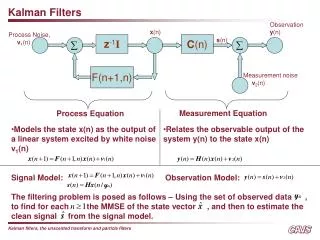
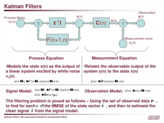
Kalman Filters. Observation y (n). x (n). Process Noise, v 1 (n). z -1 I. C (n). F(n+1,n). Measurement process v 2 (n). Measurement Equation. Process Equation. Models the state x(n) as the output of a linear system excited by white noise v 1 (n).

E N D
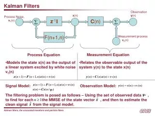
Kalman Filters Observation y(n) x(n) Process Noise, v1(n) z-1I C(n) F(n+1,n) Measurement process v2(n) Measurement Equation Process Equation • Models the state x(n) as the output of a linear system excited by white noise v1(n) • Relates the observable output of the system y(n) to the state x(n) • Signal Model: Observation Model: • The filtering problem is posed as follows – Using the set of observed data , • to find for each the MMSE of the state vector , and then to estimate the clean signal from the signal model.
Unscented Kalman Filters (motivation – where Extended Kalman filters fail) • Nonlinear State Estimation • Predicting state vector, • Kalman gain, • Predicting observation • When propagating a GRV through a linear model (Kalman filtering), it is easy to compute the expectation E[ ] • However, if the same GRV passes through a nonlinear model, the resultant estimate may no longer be Gaussian – calculation of E[ ] no longer is easy! • It is in the calculation of E[ ] in the recursive filtering process that we now need to estimate the pdf of the propagating random vector • Extended Kalman Filter (EKF) avoids this by linearizing the state-space equations and reducing the estimate equations to point estimates instead of expectations • In EKF, the state distributions are approximated by a GRV and propagated analytically through a ‘first-order linearization’ of the nonlinear system • The approximations can introduce large errors in true posterior means and covariance matrices. Vector Functions
Unscented Kalman Filters (UKFs) • Instead of propagating a GRV through the linearized system, the UKF technique focuses on an efficient estimation of the statistics of the random vector being propagated through a nonlinear function • Consider a nonlinearity • To compute the statistics of , we ‘cleverly’ sample this function using ‘deterministically’ chosen 2L+1 points about the mean of x • Can be proved that with these as sample points, the following ‘weighted’ sample means and covariance matrices will be equal to the true values • We use this set of equations to predict the states and observations in the nonlinear state-estimation model. The expected values E[ ] and the covariance matrices are replaced with these sample ‘weighted’ versions. Sigma Points
Unscented Kalman Filters (UKFs) vs. Particle Filters (PFs) • The unscented transformation in UKFs allows the calculation of accurate sample means and covariance matrices using a few ‘cleverly’ chosen samples • Particle filtering techniques employ Monte-Carlo techniques to obtain an estimate of the statistics of the propagated random vector • The two techniques are very close conceptually • There is a subtle difference : in UKF based implementations, the sigma points for sampling are deterministically chosen whereas in PF based techniques, the sampling itself is done randomly • Particle Filtering is more accurate but this comes at the cost of complexity • The complexity of UKF based implementations is about the same as that of regular Kalman filters