Download
1 / 42
420 likes | 570 Views
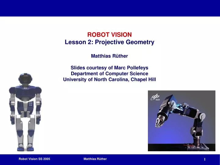
ROBOT VISION Lesson 2: Projective Geometry Matthias Rüther Slides courtesy of Marc Pollefeys Department of Computer Science University of North Carolina, Chapel Hill. Content. Linear Algebra : basic vector and matrix operations

E N D
ROBOT VISIONLesson 2: Projective GeometryMatthias RütherSlides courtesy of Marc Pollefeys Department of Computer ScienceUniversity of North Carolina, Chapel Hill
Content • Linear Algebra: basic vector and matrix operations • Background: Projective geometry (2D, 3D), Parameter estimation, Algorithm evaluation. • Single View: Camera model, Calibration, Single View Geometry. • Two Views: Epipolar Geometry, 3D reconstruction, Computing F, Computing structure, Plane and homographies. • Three Views: Trifocal Tensor, Computing T. • More Views: N-Linearities, Multiple view reconstruction, Bundle adjustment, auto-calibration, Dynamic SfM, Cheirality, Duality
Vector Basics v x2 x1 v‘ v v+v‘ w Φ v
Vector Spaces • Linear combination • Given vectors v1, ..., vkand scalars c1, ..., ck, the vector v = c1v1+ c2v2+ . . . + ckvk is obtained as a linear combination of the vectors v1, ..., vk • Example: all vectors in R3 are linear combinations of i = (1, 0, 0), j = (0, 1, 0), and k = (0, 0, 1) v = (a, b, c) = a(1, 0, 0) + b(0, 1, 0) + c(0, 0, 1) • Spanning • S=(v1, v2, . . . , vk ) spans a space W if every vector in W can be written as a linear combination of the vectors in S • Linear Indepedence • v1, ..., vk is linearly indepedent if c1v1+ c2v2+ . . . + ck vk= 0 implies c1= c2= . . . = ck= 0
Vector Spaces • Basis • S=(v1, ..., vk) is a basis for a vector space W if • vjare linearly indepedent • S spans W ! S need not be orthogonal ! • Dimension • All bases for W have the same number of vectors. • The dimension of W is the size of its sets of basis vectors. • Coordinates Relative to a Basis • If S=(v1, ..., vk) is a basis for a vector space W,then any v Î W has a unique vector expansion:
Vector Spaces • Example: • In R3 the vectors relative to and relative to are identical.
Matrix Basics • Addition/Subtraction C = A + B implies cij= aij+ bij C = A - B implies cij= aij- bij • Multiplication Cmq = Amn*Bnq implies • Determinants • det(A)=0 A is singular A is not invertible • det(A-I) is characteristic polynomial, roots are the eigenvalues
Matrix Basics • Inverse • AA-1=A-1A=I • Exists, iff det(A) != 0, A is not singular • Properties: • Pseudo-Inverse A+ = (AT A)-1AT A+A=I • Rank Maximum number of linearly independent columns or rows. • If A is mn, rank(A) <= min(m,n) • If A is nn, rank(A) = n iff A nonsingular (invertible, det(A)!=0) • If A is nn, rank(A) < n iff A singular
Solving Linear Equation Systems • Common problem: solve the equation system Amnx=b • If m>n, the system is over-determined • If m<n, the system is under-determined • If b=0, the system is homogeneous • The system has either no solutions, exactly one or infinitely many • Methods for solving Amnx=b include Gauss elimination, LU factorization, computing pseudo-inverse using SVD etc. • Conditions for solutions of Ax=b (A is square) • If A is invertible, Ax=b has exactly one solution. • A is invertible Ax=0 has only trivial solution det(A)!=0 b is in the column space of A rank(A)=n, rank(A|b)=n column/row vectors are lin. Independent column/row vectors span Rn • If b not in column space of A (rank(A|b)>rank(A)), the system has no solution • If rank(A)<n, and rank(A|b)=rank(A), the system has infinite number of solutions • Ax=0 has non-trivial solutions iff rank(A)<n
Projective 2D Geometry • Points, lines & conics • Transformations & invariants • 1D projective geometry and the Cross-ratio
x x p1 p1 p2 p2 p3 p3 p4 p4 1D Projective Geometry ℝ1 • Euclidean 1D vector space: • Geometric Primitives: points • Representation: 1D vector: p = (x) • Transformations: • Translation: p‘ = (x+t) • Scaling: p‘ = (s*x) • Translation and Scaling: p‘ = (s*x+t) dp1p2 x p‘1 p‘2 p‘3 p‘4 x p‘1 p‘2 p‘3 p‘4
1D Projective Geometry ℙ1 • 1D Projective space: Representation: 1D vector: p‘ = (x‘ w‘)T, where p = (x/w) e.g. p‘ = (2 1)T = (4 2)T = (1 0,5)T are all equivalent to p = (2) w W=1 p1 p2 p3 p4 x
1D Projective Geometry • 1D Projective space: • Geometric Primitives: points • Representation: 1D vector: p = (x w)T • Transformations: • Translation: p‘ = T * p 1DOF • Scaling: p‘ = S * p 1DOF • Translation and Scaling: p‘ = M * p, where M=S*T 2DOF • Projective Mapping: p‘ = P * p, where P is a 2x2 Matrix 3DOF
1D Projective Geometry • Translation: w W=1 p‘1 p‘2 p‘3 p‘4 x
1D Projective Geometry • Scaling: w p‘1 p‘2 p‘3 p‘4 W=1 x
1D Projective Geometry • Projective Mapping: p‘1 w p‘2 p‘3 p‘4 W=1 x Analogy to central projective camera!
1D Projective Geometry • Invariants: • transformations form a hierarchy, some geometric features remaing unchanged under the transformations • Translation (isometry) • Length, overall scale • Translation and Scaling (similarity) • Ratio of lengths (d12 : d23) • Projective Mapping (projectivity) • Cross ratio (ratio of ratios): d12*d34 = d13*d24
Homogeneous representation of points on if and only if Homogeneous coordinates but only 2DOF Inhomogeneous coordinates Homogeneous coordinates Homogeneous representation of lines equivalence class of vectors, any vector is representative Set of all equivalence classes in R3(0,0,0)T forms P2 The point x lies on the line l if and only if xTl=lTx=0
Line joining two points The line through two points and is Points from lines and vice-versa Intersections of lines The intersection of two lines and is Example
tangent vector normal direction Example Ideal points Line at infinity Ideal points and the line at infinity Intersections of parallel lines Note that in P2 there is no distinction between ideal points and others
A model for the projective plane exactly one line through two points exaclty one point at intersection of two lines
Duality principle: To any theorem of 2-dimensional projective geometry there corresponds a dual theorem, which may be derived by interchanging the role of points and lines in the original theorem Duality
or homogenized or in matrix form with Conics Curve described by 2nd-degree equation in the plane 5DOF:
or stacking constraints yields Five points define a conic For each point the conic passes through
Tangent lines to conics The line l tangent to C at point x on C is given by l=Cx l x C
In general (C full rank): Dual conics A line tangent to the conic C satisfies Dual conics = line conics = conic envelopes
Note that for degenerate conics Degenerate conics A conic is degenerate if matrix C is not of full rank e.g. two lines (rank 2) e.g. repeated line (rank 1) Degenerate line conics: 2 points (rank 2), double point (rank1)
Theorem: A mapping h:P2P2is a projectivity if and only if there exist a non-singular 3x3 matrix H such that for any point in P2 reprented by a vector x it is true that h(x)=Hx Definition: Projective transformation or 8DOF Projective transformations Definition: A projectivity is an invertible mapping h from P2 to itself such that three points x1,x2,x3lie on the same line if and only if h(x1),h(x2),h(x3) do. projectivity=collineation=projective transformation=homography
Mapping between planes central projection may be expressed by x’=Hx (application of theorem)
Removing projective distortion select four points in a plane with know coordinates (linear in hij) (2 constraints/point, 8DOF 4 points needed) Remark: no calibration at all necessary, better ways to compute (see later)
Transformation for conics Transformation for dual conics Transformation of lines and conics For a point transformation Transformation for lines
A hierarchy of transformations Projective linear group Affine group (last row (0,0,1)) Euclidean group (upper left 2x2 orthogonal) Oriented Euclidean group (upper left 2x2 det 1) Alternative, characterize transformation in terms of elements or quantities that are preserved or invariant e.g. Euclidean transformations leave distances unchanged
orientation preserving: orientation reversing: Class I: Isometries (iso=same, metric=measure) 3DOF (1 rotation, 2 translation) special cases: pure rotation, pure translation Invariants: length, angle, area
Class II: Similarities (isometry + scale) 4DOF (1 scale, 1 rotation, 2 translation) also know as equi-form (shape preserving) metric structure = structure up to similarity (in literature) Invariants: ratios of length, angle, ratios of areas, parallel lines
Class III: Affine transformations 6DOF (2 scale, 2 rotation, 2 translation) non-isotropic scaling! (2DOF: scale ratio and orientation) Invariants: parallel lines, ratios of parallel lengths, ratios of areas
Class VI: Projective transformations 8DOF (2 scale, 2 rotation, 2 translation, 2 line at infinity) Action non-homogeneous over the plane Invariants: cross-ratio of four points on a line (ratio of ratio)
Action of affinities and projectivities on line at infinity Line at infinity stays at infinity, but points move along line Line at infinity becomes finite, allows to observe vanishing points, horizon,
Decomposition of projective transformations decomposition unique (if chosen s>0) upper-triangular, Example:
Overview of transformations Concurrency, collinearity, order of contact (intersection, tangency, inflection, etc.), cross ratio Projective 8dof Parallellism, ratio of areas, ratio of lengths on parallel lines (e.g midpoints), linear combinations of vectors (centroids). The line at infinity l∞ Affine 6dof Ratios of lengths, angles. The circular points I,J Similarity 4dof Euclidean 3dof lengths, areas.
Number of invariants? The number of functional invariants is equal to, or greater than, the number of degrees of freedom of the configuration less the number of degrees of freedom of the transformation e.g. configuration of 4 points in general position has 8 dof (2/pt) and so 4 similarity, 2 affinity and zero projective invariants