X-Ray Analysis

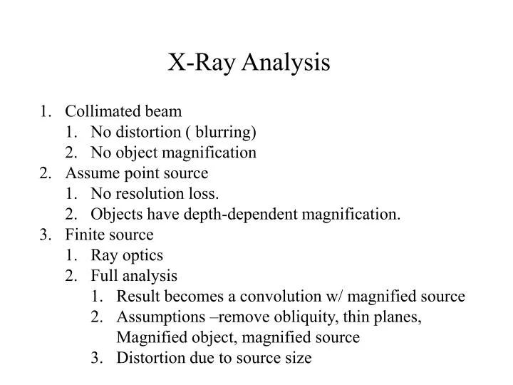
1. X-Ray Analysis • Collimated beam • No distortion ( blurring) • No object magnification • Assume point source • No resolution loss. • Objects have depth-dependent magnification. • Finite source • Ray optics • Full analysis • Result becomes a convolution w/ magnified source • Assumptions –remove obliquity, thin planes, Magnified object, magnified source • Distortion due to source size

2. Collimated X-ray Id (xd,yd) = I0 exp [ - ∫ µo (x,y,z) dz] X-Ray with a Point Source Id (xd,yd) = Ii exp [ - ∫ µo ((xd/d)z, (yd/d)z, z) dz] Id (xd,yd) = Ii exp [ - ∫ µo (xd/M, (yd/M, z) dz] where M = d/z and Ii = Io/ (1 + (rd2/d)2)3/2

3. Planar Object Geometric optics predicts that for a thin object: t (x,y) = exp [ -µ (x,y)  (z - zo)] imaged by a x-ray source, s(x,y) The detected image will be the convolution of a Magnified object and a magnified source

4. xd,yd rds xs,ys ds s(xs,ys) • • origin First, no object dId (xd, yd) = dIo cos3 dIo = s (xs, ys) dxs dys/(4πd2) Source units ((N/mm2)/min) Detailed Analysis

5. 2) Now let’s put in an object. What is the output of xd, yd given a source at xs, ys? We call this the differential detected image. dId (xd, yd, xs, ys) = dIi exp [ - ∫ µ (x,y,z) ds] Again, we will evaluate ds in terms of xd, yd in the detector plane. Nowcome up for expressions for x and y paths in terms of z

6. We want to describe what is happening at some general location x,y in the body. Let’s start by describing the coordinates of these points along a path connecting an arbitrary source point and detector point. Our source point will be s(xs,ys) and the detector point will be (xd, yd). A general point y on the path is shown. By similar triangles, X-ray path yd y ys ys µ (x,y,z) z d y-z plane shown

7. Again, we will build a parametric equation

8. Let’s manipulate one of the variables of µ in last slide, recalling that Now we have the result at an arbitrary detector point due to and arbitrary source point.

9. To get the entire result Id (xd, yd), we add up the response from all the source points by integrating over the source. Id (xd, yd) = ∫ ∫ dIs  integrate over source No assumptions made on space invariance yet. Putting it all together, Id (xd, yd) = 1/ (4πd2) ∫ ∫ s (xs, ys) exp[- ∫µ (xd - mxs)/M, (yd - mys)/M, z) dz] Let’s make some assumptions and simplify Ignore both obliquity factors Assume planar object µ =  (x,y)  (z - zo)

10. Then Id = 1/(4πd2) ∫ ∫ s (xs, ys) exp[ -  (xd - mxs)/M, (yd - mys)/M) dxs dys] For space invariance, let By considering a magnified source and Magnified object, we can get space invariance. The above can be viewed as a convolution. Id = 1/(4πd2m2) s (xd/m, yd/m) ** exp[ - (xd/M, yd/M)] Id = 1/(4πd2m2) s (xd/m, yd/m) ** t (xd/M, yd/M)]

11. Consider 10mm object 1mm source

12. Intuitive Understanding of Finite Source Instead of a point source, let’s consider a more realistic finite source. The source will be planar and parallel to the detector. We will consider it as an array of point sources. Here we will consider half a doughnut as an example, s(xs,ys). ys xd xs yd Image of Source s(xs,ys) d-z Find the result in the detector plane ss a result of the sum of source points z d

13. Geometric Ray Optics Low m Response to pinhole impulse at origin Planar Object In the Fourier domain, Id (u,v) = KM2m2 T (Mu, Mv) S (mu,mv)

14. small m Large m u z < d Geometric Ray Optics Low m In the Fourier domain, Id (u,v) = KM2m2 T (Mu, Mv) S (mu,mv) Object is magnified by Source causes distortion Id (u,v) Curves show S(mu,mv) for a large m and a small m

15. Volumetric Object What about volumetric objects? Stepping back one or two steps in the previous work and still ignoring obliquity, But m = m(z) therefore we can’t model Let’s model object as an array of planes (||||||)  (x,y) µ = ∑ i (x,y)  (z - zi) i where mi = - (d - zi)/ zi and Mi= d/zi

16. term is still not linear however Let’s assume ∫ µ dz = ∑ i << 1 Then we can linearize the exponent exp (- ∑ i) = 1 - ∑ i View as sum of integrals Id ≈ Ii - ∑i 1/(4πd2m2) s ((xd/mi), (yd/mi)) **i(xd/Mi, yd/Mi) where Ii = 1/(4πd2) ∫ ∫ s (xs,ys) dxs dys The output is seen as incident radiation minus a summation of convolutions. Good math, poor approximation. This is true only in very thin regions of the body

17. Reasonable approximation (except at boundaries u approaches 0 ) µ = µmean + µD µ∆ is departure from water or exp [ - ∫ (µm + µ∆) dz = exp [ - ∫ µm dz ] exp [ - ∫ µ∆ dz ] We can linearize with the approximation ≈[ exp - ∫ µm dz ] [ 1 - ∫ µ∆ dz ] Since µm is a constant, the first exponential term is a constant.

18. Since µm is a constant, we can pull out the first exponential term. The remaining integration can now be seen as a series of thin planes. Each plane’s integration in z is simply seen as a convolution then. Id = [exp - ∫ µm (xd/M, yd/M, z) dz ] • [ Ii - ∑ 1/(4πd2mi2) s ((xd/mi), (yd/mi)) ** ∆i (xd/Mi, yd/Mi) Id = Twater (xd, yd) [ Ii - ∑ 1/(4πd2mi2) • s ((xd/mi), (yd/mi)) ** ∆i (xd/Mi, yd/Mi)] where Twater = [exp - ∫ µm (xd/M, yd/M, z) dz ] Thus, we have justified viewing the body as an array of planes.