Download
1 / 23
300 likes | 646 Views
Quantitative X-Ray Analysis. Introduction: It is extremely important to grasp the underlying physical principles to become a sophisticated analyst rather than a mere user.

E N D
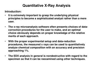
Quantitative X-Ray Analysis Introduction: • It is extremely important to grasp the underlying physical principles to become a sophisticated analyst rather than a mere user. • The x-ray microanalysis software often presents choices of data-correction procedures for the user to make, and an optimal choice obviously depends on proper knowledge of the relative merits of each approach. • With the proper experimental setup and data-reduction procedures, the measured x rays can be used to quantitatively analyze chemical composition with an accuracy and precision approaching 1%. • The EDX analysis in general is nondestructive with regard to the specimen so that it can be reexamined using other techniques.
Some key points : • As shown in Chapter 3, x rays can be generated depending on the initial electron-beam energy and atomic number, from volumes with linear dimensions as small as 1 micrometer. • This means that, typically, a volume as small as 10-12 cm3 can be analyzed. Assuming a typical density of 7 g/cm3 for a transition metal, the composition of 7 x 10-12 g of material can be determined. • From this small mass of the sample selected by the electron x-ray interaction volume, elemental consitituents can be determined to concentrations ranging as low as 0.01% (100 ppm), which corresponds to limits of detection in terms of mass of 10-16 to 10-15 g. For instance, a single atom of iron weighs about 10-22 g, so the limit of detection corresponds to only a few million atoms.
Basic Procedures for the Quantitative X-Ray Analysis • Obtain the x-ray spectrum of the specimen and standards under defined and reproducible conditions. • Measure standards containing the elements that have been identified in the specimen (a homogeneous steel sample characterized by bulk analytical chemistry procedures is ok, but a simple stoichiometric compound such as GaP is even better). • For the new EDX software, no need to remove the background since the computer will do it automatically for you.
4. Perform quanta calibration: This procedure is to develop the x-ray intensity ratios using the specimen intensity and the standard intensity for each element present in the sample and carry out matrix corrections to obtain quantitative concentration values.
The First Approximation to Quantitative Analysis • The assumption that ratio of the measured unknown-to-standard intensities, Ii/I(i) and the ratio of concentrations between the specimen and the standard should be equal is the basic experimental measurement that underlies all quantitative x-ray microanalysis and is called the “k-value”, i.e. Ci/C(i) = Ii/I(i) = k • However, careful measurements performed on homogeneous substances of known multi-element composition compared to pure element standards reveal that there are significant systematic deviations between the ratio of measured intensities and the ratio of concentrations. • Therefore, to achieve this assumption the quanta calibration has to be performed so that it would correct the matrix or inter-element effects.
Deviations between the Ratio of Measured Intensities and the Ratio of Concentrations
ZAF Matrix Correction • In mixtures of elements, matrix effects arise because of differences in elastic and inelastic scattering processes and in the propagation of x rays through the specimen to reach the detector. For conceptual as well as calculation reasons, it is convenient to divide the matrix effects into those due to atomic number, Zi; x-ray absorption, Ai; and x-ray fluorescence, Fi.
ZAF Matrix Correction Using these matrix effects, the most common form of the correction equation is Ci/C(i) = [ZAF]i Ii/I(i) = [ZAF]i ki Where Ci is the weight fraction of the element I of interest in the sample and C(i) is the weight fraction of i in the standard. This equation must be applied separately for each element present in the sample. The Z. A. and F effects must therefore be calculated separately for each element. Above equation is used to express the matrix effects and is the common basis for x-ray microanalysis in the SEM.
Effect of Atomic Number • The x-ray generation volume decreases with increasing atomic number. This is due to an increase in elastic scattering with atomic number, which deviates the electron path from the initial beam direction, and an increase in critical excitation energy Ec, with a corresponding decrease in overvoltage (U=Eo/Ec) with atomic number. • The decrease in U decreases the fraction of the initial electron energy available for the production of characteristic x rays and the energy range over which x rays can be produced. • As illustrated from the Monte Carlo simulations, the atomic number of specimen strongly affects the distribution of x-rays generated in specimens. The effects are even more complex when considering the more interesting multi-element samples as well as in the generation of L and M shell x-ray radiation.
(z) is used to evaluated the intensity of x-ray generated with the change of the escape depth of the x-ray. So (z) is a normalized generated intensity. The term z is called the mass depth and is the product of the density of the sample and the depth dimension z; is usually given in units of g/cm2.
X-Ray Absorption Effect The following figure shows that Cu characteristic x-rays are generated deeper in the specimen and the x-ray generation volume is larger as Eo increases. This is because the energy of the backscattered electrons increases with higher values of Eo.
In specimens of high atomic number, the electrons undergo more elastic scattering per unit distance and the average scattering angle is greater, as compared to low-atomic-number materials. The electron trajectories in high-atomic-number materials thus tend to deviate out of the initial direction of travel more quickly and reduce the penetration into the solid. The shape of the interaction volume also changes significantly as a function of atomic number. Effects of Atomic Number on the Distribution of X-Ray Generation
As the angle of tilt of a specimen surface increases (i.e., the angle of the beam relative to the surface decreases), the interaction volume becomes smaller and asymmetric. Influence of Specimen Surface Tilt on Interaction Volume
Thin Specimen Technique for Biological Specimen • Biological or polymer specimen is sensitive to the incident beam and very likely to be damaged by the e-beam. • The specimen structure may be rearranged. • The light elements may be evaporated while heavy elements of interest in biological microanalysis (e.g., P, S, Ca) remain. • Thin specimen technique: is based on the fact that the rate of energy loss in a low-atomic-number target is about 0.1eV/nm, so that only 10-100eV is lost through a 100-nm section.
Bulk Targets and Analysis of a Minor Element • Since the density and average atomic number of biological and many polymeric specimens is low, the excitation volume for x-rays is large. This volume can easily exceed 10 um in extent. Consequently, one of the major advantages of the method is diminished, the ability to analyze very small volumes. • In general, the increased excitation volume is acceptable to perform a ZAF analysis.
Analysis Geological Specimen • Almost all specimens for geological analysis are coated with a thin layer of C or metal to prevent surface-charging effects. However, x-rays are generated in depth in the specimen, and the surface conducting layer has no influence on electrons that are absorbed micrometers into the specimen. Electrical fields may be built up deep in the specimen, which can ultimately affect the shape of the (z) Curves. • Most geologists don’t measure oxygen directly, but get their oxygen values by stoichiometry. If oxygen analysis is desired, then C coatings are not optimal because they are highly absorbing for both O and N K x-ray.
Light-Element Analysis Quantitative x-ray analysis of the low-energy (<0.7 keV) K lines of the light elements is difficult in the SEM. The following table lists the low-atomic-number elements considered in this section along with the energies and wavelengths of the K lines. X-ray analysis in this energy range is a real challenge for the correction models developed for quantitative analysis since a large absorption correction is usually necessary. Unfortunately, the mass absorption coefficients for low-energy x-rays are very large and the values of many of these coefficients are still not well known. The low-energy x-rays are measured using large d spacing crystals in a WDS system or thin-window or windowless EDS detector.
Operation Conditions for Light-Element Analysis • One can reduce the effect of x-ray absorption by analyzing at high take-off angles and low electron-beam energies Eo. The higher the take-off angle, the shorter the path length for absorption within the specimen. The penetration of the electron beam is decreased when lower operating energies are used, and x-rays are produced closer to the surface.Figure 9.33 shows the variation of boron K intensity with electron-beam energy Eo, at a constant take-off angle for boron and several of its compounds. A maximum in the boron K intensity occurs when Eo is 5 to 15 keV, depending on the sample.