Download

1 / 61
630 likes | 838 Views
Forecasting convective rainfall: convective initiation, heavy precipitation and flash flooding. Robert Fovell University of California, Los Angeles rfovell@ucla.edu. Heavy precipitation at a location = intensity + longevity. Common sources of heavy precipitation in U.S.

E N D
Forecasting convective rainfall:convective initiation, heavy precipitation and flash flooding Robert Fovell University of California, Los Angeles rfovell@ucla.edu
Common sources of heavy precipitation in U.S. • Mesoscale convective systems and vortices • Orographically induced, trapped or influenced storms • Landfalling tropical cyclones
MCSs & precipitation facts • Common types: squall-lines and supercells • Large % of warm season rainfall in U.S. and flash floods (Maddox et al. 1979; Doswell et al. 1996) • Initiation & motion often not well forecasted by operational models (Davis et al. 2003; Bukovsky et al. 2006) • Boundary layer, surface and convective schemes “Achilles’ heels” of regional-scale models • Improved convective parameterizations help simulating accurate propagation (Anderson et al. 2007; Bukovsky et al. 2006) • Supercells often produce intense but not heavy rainfall • Form in highly sheared environments • Tend to move quickly, not stay in one place
Seasonality of flash floods in U.S. Contribution of warm season MCSs clearly seen Number of events Maddox et al. (1979)
Linear MCS archetypes(e.g., squall-lines) 58% 19% 19% Parker and Johnson (2000)
The multicell storm Four cells at a single time Or a single cell at four times: unsteady Browning et al. (1976)
The multicell storm Unsteadiness = episodic entrainment owing to local buoyancy-induced circulations. Browning et al. (1976) Fovell and Tan (1998)
Storm motion matters How a storm moves over a specific location determines rainfall received Doswell et al. (1996)
Storm motion matters Doswell et al. (1996)
Forecasting MCS motion (or lack of motion…)
Some common “rules of thumb” ingredients • CAPE (Convective Available Potential Energy) • CIN (Convective Inhibition) • Precipitable water • Vertical shear - magnitude and direction • Low-level jet • Midlevel cyclonic circulations
Some common “rules of thumb” • MCSs tend to propagate towards the most unstable air • 1000-500 mb layer mean RH ≥ 70% • MCSs tend to propagate parallel to 1000-500 mb thickness contours • MCSs favored where thickness contours diverge • MCSs “back-build” towards higher CIN • Development favored downshear of midlevel cyclonic circulations
70% layer RH 70% RH rule of thumb Implication: Relative humidity more skillful than absolute humidity RH > 70% # = precip. category Junker et al. (1999)
MCSs tend to follow thickness contours Implication: vertical shear determines MCS orientation and motion. Thickness divergence likely implies rising motion
Back-building towards higher CIN Lifting takes longer where there is more resistance
Corfidi vector method Propagation is vector difference P = S - C Therefore, S = C + P
Schematic example We wish to forecast system motion So we need to understand what controls cell motion and propagation
Individual cell motion • “Go with the flow” • Agrees with previous observations (e.g, Fankhauser 1964) and theory (classic studies of Kuo and Asai) Cells tend to move at 850-300 mb layer wind speed* *Layer wind weighted towards lower troposphere, using winds determined around MCS genesis. Later some slight deviation to the right often appears Corfidi et al. (1996)
Individual cell motion Cell direction comparable To 850-300 mb layer wind direction Cells tend to move at 850-300 mb layer wind speed Corfidi et al. (1996)
Composite severe MCS hodograph Bluestein and Jain (1985)
Composite severe MCS hodograph Low-level jets (LLJs) are common Note P ~ -LLJ Bluestein and Jain (1985)
Propagation vector and LLJ • Many storm environments have a low-level jet (LLJ) or wind maximum • Propagation vector often anti-parallel to LLJ Propagation vector direction P ~ -LLJ Corfidi et al. (1996)
Forecasting system motionusing antecedent information Cell motion ~ 850-300 mb wind Propagation ~ equal/opposite to LLJ S = C - LLJ
Evaluation of Corfidi method Method skillful in predicting system speed and direction Corfidi et al. (1996)
Limitations to Corfidi method • Wind estimates need frequent updating • Influence of topography on storm initiation, motion ignored • Some storms deviate significantly from predicted direction (e.g., bow echoes) • P ~ -LLJ does not directly capture reason systems organize (shear) or move (coldpools) • Beware of boundaries! • Corfidi (2003) modified vector method
5 June 2004 X = Hays, Kansas, USA
Cyclonic vortex following squall line Not a clean MCV case
Potential vorticity (PV) anomalies PV anomaly shown drifting in westerly sheared flow Raymond and Jiang (1990)
Potential vorticity (PV) anomalies Ascent occurs on windward (here, east) side… destabilization Raymond and Jiang (1990)
Potential vorticity (PV) anomalies Cyclonic circulation itself results in ascent on east side Raymond and Jiang (1990)
Potential vorticity (PV) anomalies Combination: uplift & destabilization on windward side AND downshear side Raymond and Jiang (1990)
Composite analysis of MCV heavy rain events • Based on 6 cases poorly forecasted by models • Composite at time of heaviest rain (t = 0h) • Heaviest rain in early morning • Heaviest rain south of MCV in 600 mb trough 600 mb vorticity (color), heights and winds. Map for scale only Schumacher and Johnson (2008)
Schumacher’s situation “Hairpin” hodograph: Sharp flow reversal above LLJ
Schumacher’s situation South side of MCV is windward at low-levels and downshear relative to midlevel vortex
Back-building Ground-relative system speed ~ 0 Schumacher and Johnson (2005) Doswell et al. (1996)
Evolution of the heavy rain event At t - 12h (afternoon): - MCV located farther west - 900 mb winds fairly light 600 mb vorticity, 900 mb winds & isotachs Schumacher and Johnson (2008)
Evolution of the heavy rain event At t - 6h (evening): - MCV drifted west - 900 mb winds strengthening (LLJ intensifying) 600 mb vorticity, 900 mb winds & isotachs Schumacher and Johnson (2008)
Evolution of the heavy rain event At time of heaviest rain (midnight): - 900 mb jet well developed - LLJ located east, south of MCV 600 mb vorticity, 900 mb winds & isotachs Schumacher and Johnson (2008)
Evolution of the heavy rain event At t + 6h (morning): rain decreases as LLJ weakens 600 mb vorticity, 900 mb winds & isotachs Schumacher and Johnson (2008)
Episodes of MCSs & predictability Hovmoller diagrams reveal westward- propagating MCSs Note “envelope” of several systems with “connections” Carbone et al. (2002)
MCV role in predictability Carbone et al. (2002)
“Training lines” of cells • In Asia, stationary front could be the Mei-Yu (China), Baiu (Japan) or Changma (Korea) front • Motion along the front and/or continuous back- building Schumacher and Johnson (2005)
Record 619 mm in 15 h at Ganghwa, Korea X shear Lee et al. (2008) Sun and Lee (2002)