Download
1 / 55
550 likes | 556 Views
Geology 659 - Quantitative Methods. Basic Statistics Review. tom.h.wilson wilson@geo.wvu.edu. Department of Geology and Geography West Virginia University Morgantown, WV. Statistical Characterization of Data. Rock property assessment.

E N D
Geology 659 - Quantitative Methods Basic Statistics Review tom.h.wilson wilson@geo.wvu.edu Department of Geology and Geography West Virginia University Morgantown, WV
Statistical Characterization of Data Rock property assessment Consider the attributes that you might use to describe a rock such as grain size, porosity, composition (percent quartz, orthoclase, …), dip, etc. How are these different attributes obtained? How reliable are the values that are reported?
Concepts and terminology - Specimen - a part of a whole or one individual of a group. Sample - several specimens Population - all members of the group, all possible specimens from the group
Concepts and terminology - The attributes derived form the sample are referred to as statistics. The attributes derived from the entire population of specimens are referred to as parameters.
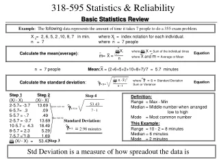
Consider your grade in a class - Let’s say that your semester grade is based on the following 4 test scores. 85, 80, 70 and 95. What is your grade for the semester? You grade is the average of these 4 test scores or 82.5
The average is often used to represent the most likely value to be encountered in a sample or population. Is the average grade of 82.5 a statistic or a parameter? Since the entire population of grades for the student consists of just those 4 test scores, their average score is a parameter.
Pebble Masses At left is a table of masses (in grams) of 100 pebbles taken from a beach. The average mass of these pebbles is 350.18 grams This average is a ... statistic
Computation of the mean or average In this equation mi is the mass of pebble i N is the total number of specimens i ranges from 1 to N m = the average mass of all the pebbles in the sample.
If we draw smaller samples at random from our original sample of 100 specimens and then compute their averages, we begin to appreciate that the statistical average is only an estimate of the population average.Recall that the mean estimated from 100 samples was 350.18. <average> = 355.1g
Other measures of the most common value in a population include the median and the mode. If we sort measured values (for example pebble mass) in increasing order, from the lightest pebble to the heaviest and look at the mass of the center pebble, that value is the median mass.
In the sample (1,2,3,4,5) - 3 is the center or median value of the sample. In the sample 1,2,3,4 we have an even number of observations and in this case the median is taken as the average of the middle two values or 2.5.
At right, the pebble mass has been sorted in ascending order from the lightest to heaviest pebbles in the sample. There are an even number of specimens in this sample, so the median must be determined from the average of specimens 50 and 51 Median =352.5 g
Mode The mode is the value that occurs most frequently. For example, in the following sample, (1,2,2,3,3,3,4,5), 3 occurs most frequently and would be the mode of this sample.
In the sample of rock masses, 283, 331, 338, 355 and 403 all occur 3 times. We cannot define a single mode.
The Histogram - a graphical display of the distribution of values.
The appearance of the histogram will vary depending on the specified range you use to subdivide the sample values. You might group your samples into 25 gram ranges extending from 226 through 250, 251 through 275 and so on.
Or 50 gram intervals - The median is 352.5 grams and the mean 350.18 grams
The distribution of masses from beach B is similar in shape to that from our first beach, but its range is much smaller. Both samples have the same mean.
A The pebbles on beach B are much better sorted than those on beach A. There is not as much variation in pebble mass on beach B.
Sample B is better sorted than our first sample. The mass distribution below has the same range as distribution B and nearly the same mean (348 grams), but its shape is very different. This distribution is much more irregularly distributed across the range - i.e. there’s not a preferred value.
A parameter that describes the spread or dispersion in the values of a population is its variance. Note the brackets indicate that we are taking the mean or average of this quantity. 2 is used to represent the population variance
The statistic used to quantify the spread or dispersion in the values of a sample is the sample variance. The sample variance is computed in the following way - s2 represents the sample variance
The standard deviation of the sample values is a statistic that is also often used to describe the degree of variation in values of a sample. The standard deviation is just the square root of the variance.
Standard deviation =32.37 Standard deviation =23.83 While these two distributions have similar means, the one on the right is better sorted and, the standard deviation - not the range - reveals this difference.
The standard deviation describes geological differences in the sample that are not apparent in their means. One sample is better sorted - has smaller standard deviation than the other, which is less sorted and has higher standard deviation.
Note - The sample variance is considered to be an underestimate of the population variance or actual variance of the parent population. To compensate for that, and to obtain an estimate of the population variance which is considered more accurate, the sample variance is corrected to form an “unbiased ” estimate of the population variance.
The following equation is used to compute the unbiased estimate of the population variance -
Probability Probability can be thought of as describing that fraction of all possible values that a specific value or range of values will be observed out of the total number of observations or specimens in a sample. Just as with the average and the standard deviation, there is a distinction between the probabilities associated with a sample and those of the parent population….
The probabilities observed in the sample give one an estimate of the probability or likelihood of occurrence in the parent population. Probabilities are used to make predictions as well as for characterization.
Note that the probability of individual occurrences may vary. The probability that you will get a pebble with a mass of 242 grams is one in a hundred. The probability of picking up a pebble that has a 283 gram mass is 3 in 100 (0.03), etc.
The probability that a pebble will have a mass somewhere in the range 300 to 350 will be 35 out of 100 or 0.35.
These probabilities are the probabilities that individual values in a sample will fall in a 50 gram range, and thus represent the integral of individual probability over the range.
Probability distributions with a shape similar to the above example are quite common. They are nearly symmetrical and values near the average are more probable than those further from the average.
Distributions of this type are often referred to as Gaussian or normal distributions. And we can estimate the probability distribution of the parent population from statistical estimates of the mean and variance.
This expression is often simplified by substituting Z for (x-x)/. Z is referred to as the standard normal deviate, and the Gaussian distribution is rewritten as - Note that (x-x)/ represents the number of standard deviations the value x is from the mean value.
Thus a value x corresponding to a z of 2 would be located two standard deviations from the mean in the positive direction. Using the pebble mass statistics, <x>=350.18 and s=48. Thus a specimen with z of 2 implies that its mass x = 446 grams.
The Gaussian (normal) distribution of pebble masses looks a bit different from the probability distribution we derived directly from the sample.
Gaussian Distribution? The probability of occurrence of specific values in a sample often takes on a bell-shaped appearance as in the case of our pebble mass distribution.
What is the equivalent probability that a pebble having a mass somewhere between 401 and 450 grams will be drawn from a normal distribution having the same mean and standard deviation as the sample.
Note that 401 grams lies (401-350)/48 or +1.06 standard deviations from the mean. 450 grams lies (450-350)/48 or +2.08 standard deviations from the mean value. 1.06 and 2.08 are z-values or the standard normal representation of the mass data.
How can we estimate the area between p (z = 1.06) and p(z=2.08) from the area table? Note that area shown above corresponds to the probability that a sample drawn at random from this population will have a value somewhere between 401 and 450 grams.
This Area Note that we can express the area (or probability) as one half the difference of areas cited in the table.
Let’s take a simpler example and determine the probability that a sample will have a value that falls between 1 and 2 standard deviations from the mean.
First read the areas beneath the normal distribution for ± 1 and ±2 standard deviations from the mean.
0.954-0.683 = 0.271 The difference equals the sum of two areas, one between -1 and -2 standard deviations from the mean and the other between 1 and 2 standard deviations between the mean.
We’re only after the area on the positive side of the bell between 1 and 2 standard deviations - so take 1/2 the difference.