Download
1 / 36
360 likes | 503 Views
Section 9.6 Linear Correlation. Objectives: 1. To see the method of least squares to determine the best-fit line through a set of data points. 2. To calculate correlation and coefficient of determination. Population of a bacteria culture after every generation. Gen Pop 1 1 2 3

E N D
Section 9.6 Linear Correlation
Objectives: 1. To see the method of least squares to determine the best-fit line through a set of data points. 2. To calculate correlation and coefficient of determination.
Population of a bacteria culture after every generation Gen Pop 1 1 2 3 3 2 4 3 5 5 6 4 7 5 6 5 4 3 2 1 Population 1 2 3 4 5 6 7 Generation
Finding the line of best fit is calledlinear regression. Correlationmeasures the strength of the relationship between two variables.
Suppose y = mx + b is the equation of the best-fit line. For each data point (xi, yi), you could calculate the predicted y-value, yi (yi-hat), by the line yi = mxi + b. ˆ ˆ
ˆ To have a good model, the yi on the best-fit line should be close to the yi of the original data for each xi.
Since the sum of the deviations will be zero, we will minimize the sum of the squared deviations.
n n ˆ (yi – yi)2 = (yi – mxi – b)2 SSE = i=1 i i=1 This method is called the method of least squares. Since the sum of the squared deviations represents the error between the line and actual data, SSE is used as an abbreviation for the sum of squares error.
n 2 x SS = ( x - ) x i i=1 n 2 SS = ( y - ) y y i i=1 n x y SS = ( x - )( y - ) xy i i i=1 You can also compute the sum of squared deviations for the x and y variables separately.
Using the method of least squares, the best - fit line SS xy y = mx + b has slope m = SS x and y - intercept b = y - m x . Theorem 9.6: Linear Regression
x = 28/7 = 4 y = 23/7 = 3.29 EXAMPLE 1 Give the equation of the line for the bacteria population. Predict the population after the eighth generation. xi = 1+2+3+4+5+6+7 = 28 yi = 1+3+2+3+5+4+5 = 23
xi yixi-x yi-y (xi-x)2 (yi-y)2 (xi-x)(yi-y) 1 1 -3 -2.29 9 5.22 6.86 2 3 -2 -0.29 4 0.08 0.57 3 2 -1 -1.29 1 1.65 1.29 4 3 0 -0.29 0 0.08 0.00 5 5 1 1.71 1 2.94 1.71 6 4 2 0.71 4 0.51 1.43 7 5 3 1.71 9 2.94 5.14 1 1 2 3 3 2 4 3 5 5 6 4 7 5 28 13.43 17.00
SS 17 xy m = = = 0.61 SS 28 x b = y - mx SSx = 28 SSy = 13.43 SSxy = 17 = 3.29 - (0.61)(4) = 0.86 y = mx + b = 0.61x + 0.86 f(8) = 0.61(8) + 0.86 = 5.71
CorrelationA measure of the strength of the relation between two variables using the formula SSxy r = SSxSSy Definition
Definition Coefficient of determination The square of the correlation, r2.
The ranges for these measures are 0 r2 1 and -1 r 1. When all the data falls exactly on the least squares line, the model has no error and SSE = 0. This means that r2 = 1 (and r = 1 or -1). If the model does not help at all, and there is no reduction in error, then SSE = SSy, making r2 = 0 (and r = 0).
A correlation of 0 means the model is worthless, and a correlation of ±1 means that it is perfect.
SSxy r = SSxSSy 17 r = 28(13.43) EXAMPLE 2 Find the correlation between generation and population size for bacteria. ≈ 0.88
Since r > 0, the positive correlation tells us that the slope of the best-fit line is positive. Since r2 = 0.77, using the line provides a 77% reduction in error over using the average, the horizontal line.
Homework pp. 477-479
Given SSx = 100, SSy = 25, SSxy = -50, y = 4, and x = 6, find 1. the slope of the best-fit line.
Given SSx = 100, SSy = 25, SSxy = -50, y = 4, and x = 6, find 2. the intercept of the best-fit line.
Given SSx = 100, SSy = 25, SSxy = -50, y = 4, and x = 6, find 3. the equation of the best-fit line.
Given SSx = 100, SSy = 25, SSxy = -50, y = 4, and x = 6, find 4. the correlation r and its meaning.
Given SSx = 100, SSy = 25, SSxy = -50, y = 4, and x = 6, find 5. the error SSE of the model.
If y = 4x + 3 is the best-fit line by the method of least squares and SSx = 2, and SSy = 71, then 6. predict y when x is 8.
If y = 4x + 3 is the best-fit line by the method of least squares and SSx = 2, and SSy = 71, then 7. find SSxy.
If y = 4x + 3 is the best-fit line by the method of least squares and SSx = 2, and SSy = 71, then 8. find r.
If y = 4x + 3 is the best-fit line by the method of least squares and SSx = 2, and SSy = 71, then 9. interpret r.
If y = 4x + 3 is the best-fit line by the method of least squares and SSx = 2, and SSy = 71, then 10. find SSE.
■ Cumulative Review: Consider the function: f(x) = x4 + 2x3 – 35x2 – 36x + 180. 31. Find the zeros of the function.
■ Cumulative Review: Consider the function: f(x) = x4 + 2x3 – 35x2 – 36x + 180. 32. Is the function even? odd? Identify any symmetry.
■ Cumulative Review: Consider the function: f(x) = x4 + 2x3 – 35x2 – 36x + 180. 33. Graph the function.
■ Cumulative Review: 34. Solve the equation x3 + 125 = 0.
■ Cumulative Review: 35. Solve the system using Cramer’s rule. 4x – 5y = 8 3x + 2y = 4