Download
1 / 29
290 likes | 390 Views
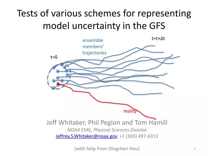
Tests of various schemes for representing model uncertainty in the GFS . t=t+Δt. ensemble members’ trajectories. t=0. reality. Jeff Whitaker, Phil Pegion and Tom Hamill NOAA ESRL, Physical Sciences Division Jeffrey.S.Whitaker@noaa.gov , +1 (303) 497-6313 (with help from Dingchen Hou ).

E N D
Tests of various schemes for representing model uncertainty in the GFS t=t+Δt ensemble members’ trajectories t=0 reality Jeff Whitaker, Phil Pegion and Tom Hamill NOAA ESRL, Physical Sciences Division Jeffrey.S.Whitaker@noaa.gov, +1 (303) 497-6313 (with help from DingchenHou)
Test hypothesis • Via a new suite of model uncertainty parameterizations (ECMWF’s SPPT, ECMWF/Met Office’s SKEB, home-grown stochastically perturbed boundary layer RH), we hypothesize that: • short and medium-range ensemble forecast spread can be increased to be more consistent with RMS error, improving probabilistic forecasts. • additive noise that is currently used to simulate model uncertainty in data assimilation can be replaced with model uncertainty parameterizations.
NCEP operational scheme (STTP)Stochastic Total Tendency Perturbation this method tends to add spread preferentially where spread already is large. Also, ensemble members are slaved together into one executable, which could mean that the whole ensemble could fail when one CPU fails. random linear combinations of ensemble tendency perturbations added to state every 6-h (entire ensemble must be run concurrently).
New schemes tested: a combination of: • Stochastically-perturbed physics tendencies (SPPT) – operational ECMWF scheme. • Stochastic kinetic energy backscatter. • Vorticity confinement (only for data assimilation experiment here) • Stochastically-perturbed boundary-layer humidity (SHUM). (some details in supplementary slides)
Test methodology • T574L64 GEFS, using new semi-Lagrangian advection. • Daily, August 1, 2013 to September 1, 2013 • 20-member ensembles. • Initialized off operational hybrid GSI/EnKF control and operational ETR perturbations. • Precipitation: used 1-degree CCPA analysis as verification. • Used blended ECMWF/NCEP analysis for validation • For comparison: • CONTROL (no model uncertainty) • STTP (operational model uncertainty method)
Day +5 RMS error / spread, temperature This ratio should be equal to 1.0, ideally. Where > 1.0, indicates a lack of spread 1.33 1.5 1.5 2.0 1.33 1.5 1.5 1.33 1.5
500 hPa height, spread and RMS error Ens. Mean RMS err Ens. Spread m m m Lead time (Days)
850 hPa temperature, spread and RMS error Ens. Mean RMS err Ens. Spread K K K Lead time (Days)
Data assimilation experiment • Control: • As in NCEP ops (using additive inflation). • Expt: • Replace additive inflation with combination of SPPT, SHUM, SKEB and VC. Spatial/temporal scales of 250km / 6 hrs for each (except 1000 km/6 hrs for VC). Stochastic VC. Amplitudes set to roughly match additive inflation spread. Multiplicative inflation as in NCEP ops. • Period: Sept 1 to Oct 15 2013, after 7 day spinup.
Conclusions • Combination of SPPT, SKEB,and SHUM improves medium-range forecast guidance substantially. • Also useful for improving treatment of model uncertainty in data assimilation. • We will work with EMC to get this implemented.
ECMWF method (SPPT)Stochastically Perturbed Physics Tendency • Perturbed Physics tendencies Original tendencies from gbphys • μ- vertical weight: 1.0 between surface and 100 hPa, decays to zero between 100 hPa and 50 hPa. • r- horizontal weights: ranges from -1.0 to 1.0, a red noise process with a • Temporal timescale of 6 hours • e-folding spatial scale of 500 km
Examples of stochastic patterns 1000 km 3 d 2000 km 30 d 500 km 6 h (from M Leutbecher)
Vorticity confinement(Sanches, Williams and Shutts, 2012 QJR doi10.1002) ε=0.6 in our experiments
Stochastic boundary-layer humidity • SPPT only modulates existing physics tendency (cannot change sign, trigger new convection). • Triggers in convection schemes very sensitive to BL humidity. • Vertical weight r decays exponentially from surface. Added every time step after physics applied. Random pattern μ has a (very small) amplitude of 0.00375, horizontal/vertical scales (250 km, 3-h).