Download
1 / 26
270 likes | 472 Views
On representing model uncertainty in climate predictions. T.N.Palmer ECMWF. with thanks to Francisco Doblas-Reyes, Thomas Jung and Antje Weisheimer, ECMWF. Initial uncertainty. Scenario uncertainty. Scenario uncertainty. Model uncertainty. Model uncertainty. Hawkins and Sutton, 2009.

E N D
On representing model uncertainty in climate predictions T.N.Palmer ECMWF with thanks to Francisco Doblas-Reyes, Thomas Jung and Antje Weisheimer, ECMWF
Initial uncertainty Scenario uncertainty Scenario uncertainty Model uncertainty Model uncertainty Hawkins and Sutton, 2009
Standard Numerical Ansatz for Climate Model Eg Increasing scale • Eg momentum“transport” by: • Turbulent eddies in boundary layer • Orographic gravity wave drag. • Convective clouds Deterministic local bulk-formula parametrisation
Towards Comprehensive Earth System Models 1970 1997 2000 1975 1985 1992 Atmosphere Atmosphere Atmosphere Atmosphere Atmosphere Atmosphere Land surface Land surface Land surface Land surface Land surface Ocean & sea-ice Ocean & sea-ice Ocean & sea-ice Ocean & sea-ice Sulphate aerosol Sulphate aerosol Sulphate aerosol Non-sulphate aerosol Non-sulphate aerosol Carbon cycle Carbon cycle Atmospheric chemistry Off-line model development Strengthening colours denote improvements in models Sulphur cycle model Non-sulphate aerosols Ocean & sea-ice model Land carbon cycle model Carbon cycle model Ocean carbon cycle model The Met.OfficeHadley Centre Atmospheric chemistry Atmospheric chemistry
1970 1997 2000 1975 1985 1992 Atmosphere Atmosphere Atmosphere Atmosphere Atmosphere Atmosphere A Missing Box Land surface Land surface Land surface Land surface Land surface Ocean & sea-ice Ocean & sea-ice Ocean & sea-ice Ocean & sea-ice Sulphate aerosol Sulphate aerosol Sulphate aerosol Non-sulphate aerosol Non-sulphate aerosol Carbon cycle Carbon cycle Atmospheric chemistry Uncertainty Off-line model development Strengthening colours denote improvements in models Sulphur cycle model Non-sulphate aerosols Ocean & sea-ice model Land carbon cycle model Carbon cycle model Ocean carbon cycle model The Met.OfficeHadley Centre Atmospheric chemistry Atmospheric chemistry
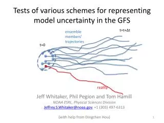
How can uncertainty be represented in ESMs? • Multi-model ensembles • Perturbed parameters • Stochastic parametrisation
Seasonal Reforecasts (months 2-4) of El Niño with a comprehensive coupled model observations predictions
Multi-model Seasonal Forecast Reliability precipitation in DJF start dates: Nov hindcast period: 1991-2005 lower tercile Amazon Central America Northern Europe Failure of multi-model ensemlble
Surface Pressure Blocking Anticyclone As recognised in AR4, the current generation of climate models has difficulty simulating a number of internal modes of climate variability such as the persistent blocking anticyclone. Potential Vorticity on 315K
Blocking Index. DJFM 1960-2003 ERA-40 T1259 T159 T1259 run on NSF Cray XT4 “Athena” (two months of dedicated usage) Similar results found by M.Matsueda MRI Japan
For all their pragmatic value, multi-model ensembles are ad hoc “ensembles of opportunity”. Component models have common shortcomings, eg due to limited resolution.
How can uncertainty be represented in ESMs? • Multi-model ensembles • Perturbed parameters • Stochastic parametrisation
Perturbed Parameters Increasing scale Deterministic local bulk-formula parametrisation Vary α
How can uncertainty be represented in ESMs? • Multi-model ensembles • Perturbed parameters • Stochastic parametrisation
A stochastic-dynamic paradigm for the Earth-System model Increasing scale Computationally-cheap nonlinear stochastic-dynamic models, providing specific possible realisations of sub-grid motions rather than sub-grid bulk effects Coupled over a range of scales ECMWF Tech Memo 598
Spectral Stochastic Backscatter Scheme • Origins: Leith (1990), Mason and Thomson (1992) • Shutts, G.J. (2005). A kinetic energy backscatter algorithm for use in ensemble prediction systems. Q.J.R.Meteorol.Soc. 131, 3079 • Berner, J. et al (2009). A spectral stochastic kinetic energy backscatter scheme and its impact on flow-dependent predictability in the ECMWF ensemble prediction system. J. Atmos.Sci., 66, 603-626. SAC 2009
Backscatter Algorithm Pattern using spectral AR(1) processes as SPPT Streamfunction forcing Dtot is a smoothed total dissipation rate, normalized here by Btot and bR is the backscatter ratio SAC2009
In ENSEMBLES we have tested the relative ability of these different representations of uncertainty:Multi-model ensemblesPerturbed parametersStochastic physicsto make skilful probabilistic seasonal climate predictions.
1991-2005 lead times: 2-4 months Dry=lower tercile Wet=upper tercile Which is best? Brier Skill Score
1991-2005 lead times: 2-4 months Cold=lower tercile Warm=upper tercile Brier Skill Score
Multi-model Seasonal Forecast Reliability precipitation over Northern Europe land (north of 48ºN) in DJF start dates: Nov 1st. hindcast period: 1991-2005 lower tercile multi-model stochastic physics #7 perturbed physics BSS(∞)=-0.031 BSS(∞)=-0.018 BSS(∞)=0.087
Conclusions • Stochastic parametrisation and perturbed parameter methodologies are competitive with the traditional multi-model approach to representing model uncertainty • Stochastic parametrisation “wins” overall for atmospheric variables, but needs to be extended to the ocean and the land surface. • The ECMWF THOR integrations will be started next year using the latest stochastic parametrisation schemes.