Download

1 / 184
1.84k likes | 1.85k Views
Model Predictive Uncertainty. Sensitivity analysis …. GM Seam Inflows. Permian Inflows. Tertiary Sands Inflow. Hydraulic property heterogeneity. correlation length. Hydraulic property correlation decreases with distance. correlation length. C(K 1 , K 2 ). distance.

E N D
Hydraulic property heterogeneity correlation length
Hydraulic property correlation decreases with distance correlation length C(K1 , K2 ) distance
Hydraulic property correlation decreases with distance correlation length variogram C(K1 , K2 ) distance
Hydraulic property correlation decreases with distance correlation length variogram C(K1 , K2 ) distance
Estimated parameter values p2 Objective function minimum p1
Estimated parameter values Objective function minimum p2 Maximum probability for p1 and p2 p1
Estimated parameter values Allowed parameter values p2 Maximum probability for p1 and p2 p1
Estimated parameter values Allowed parameter values p2 Maximum probability for p1 and p2 p1
Estimated parameter values – nonlinear case Allowed parameter values p2 Maximum probability for p1 and p2 p1
Field or laboratory measurements and model output:- Model output value calibration dataset prediction q2 q1 q3 etc distance or time
Field or laboratory measurements and model output:- Model output value Lower predictive limit calibration dataset q2 q1 q3 etc distance or time
Field or laboratory measurements and model output:- Model output value Upper predictive limit calibration dataset q2 q1 q3 etc distance or time
Field or laboratory measurements and model output:- Model output value Confidence interval for prediction calibration dataset q2 q1 q3 etc distance or time
Estimated parameter values – nonlinear case Allowed parameter values p2 Maximum probability for p1 and p2 p1
Estimated parameter values – nonlinear case knowledge constraints p2 Allowed parameter values p1
A certain model prediction p2 Increasing value p1
Defining a confidence interval p2 The critical points p1
Residuals Model output value calibration dataset prediction q2 q1 q3 etc distance or time
The variance of the residuals is:- 2 = / (m - n) m = number of observations n = number of parameters
Field or laboratory measurements and model output:- Model output value Confidence interval for prediction calibration dataset q2 q1 q3 etc distance or time
Field or laboratory measurements and model output:- Model output Predictive uncertainty interval value calibration dataset q2 q1 q3 etc distance or time
Software for predictive uncertainty analysis • UCODE • assumes model linearity • only works with a few parameters • PEST • full nonlinear predictive analysis • unlimited number of parameters
Estimated parameter values:- p2 Extreme values of p1 and p2 p1
A simple lumped parameter model par1 par2 par5 par6 par3 par4
The covariance matrix of the estimated parameter set is given by C(p) = 2 (Mt QM)-1 For a nonlinear model replace M by J, the Jacobian matrix. C(p) = 2 (Jt QJ)-1
Let M (ie. green M) represent the action of the model in predictive mode and o the model outputs in predictive mode. Then C(o) = MC(p)Mt For a nonlinear model:- C(o) = JC(p)Jt Notice that predictions can be correlated.
probability value of prediction #1
Maximum probability Bivariate probability density function.
PEST’s predictive analyzer p2 Initial parameter estimates The critical point p1
PEST’s predictive analyzer p2 The critical point Initial parameter estimates p1
Major problem with this approach • assumes that there is an objective function minimum • assumes that this defines a unique set of parameters • thus it assumes that parameters are “lumped” and that there aren’t many of them
A Confined Aquifer head Fixed Inflow T1 T3 T2 Fixed head