Download
1 / 55
550 likes | 648 Views
Ocean exchanges with the atmosphere. ….did we learn anything during WOCE?. Peter K. Taylor Southampton Oceanography Centre UK. Wind Stress. Heat Fluxes. Overview. What surface fluxes were needed for WOCE. How the flux estimates are obtained.

E N D
Ocean exchanges with the atmosphere ….did we learn anything during WOCE? Peter K. Taylor Southampton Oceanography Centre UK
Wind Stress • Heat Fluxes Overview • What surface fluxes were needed for WOCE • How the flux estimates are obtained • How far have we progressed during the WOCE period “Separately for…” • Future Flux Observing System
Need heatand freshwater fluxes Need wind stress The Goals of WOCE
The important Air-Sea fluxes for WOCE “Net heat flux is sum of…”
The important Air-Sea fluxes for WOCE “but little in this talk on precipitation since accuracy still poor”
Need climatological flux fields Need to develop Observing System Goal 2 of WOCE
Air-Sea Flux aims for WOCE • Produce estimates of the global air-seafluxes of heat, freshwater and momentumon a range of time and space scales • Produce climatological fields for these fluxes • Work toward definition of an on-going observing system for the surface fluxes
How surface fluxes are determined • Budget methods give total heat flux: • divergence of ocean heat transport (e.g. Ganachaud & Wunsch, 2000) • atmospheric flux divergence with top of atmosphere radiative balance …the “residual” method(e.g. Trenberth et al. 2001 )
Determining the individual flux components • SW and LW Radiative fluxes can be obtained from Satellite data and from NWP models • Turbulent fluxes from in situ data, models, and satellites, are based on meteorological variables (temperature, wind, etc.) and the bulk formulae
CEdepends on the roughness length(s) and stability (z / L ) Example of Bulk FormulaLatent heat flux (W/m2) Flux= Transfer x Wind x humidityCoefficient speed difference
SeaSat (1978) JASIN (1978) GATE (1974) Determining the Transfer Coefficient “SeaSat coincided with JASIN” GARP Air-Sea Interaction experiments :BOMEX, AMTEX, IFYGL
The Legacy of GARP: • Budget experiments are difficult! • Experimental data on transfer coefficients was available The Legacy of SeaSat: • Satellite scatterometers could define wind forcing • We must continue to maintain (and improve)the in situ observing systems
1.5 1.4 0.9 0.9 1.6 1.4 1.4 1.2 1.0 1.4 2.0 1.3 1.0 1.4 1.8 1.3 1.2 1.3 1.4 Developing the Voluntary Observing Ship (VOS) system • Due to research during the WOCE period (partly funded by TOGA and WOCE): • The random and systematic errors in VOS data are much better known “we can now plot a map of error values like this one” • Now greater emphasis on meta-data ….how the observations are obtained Mean random errors in ship SST obs ( C )1970 - 1997 (Kent, 2002)
Wind Stress • The choice of Drag Coefficient, CD10n • Effect of using other CD10n values • Climatic variations in mean wind stress • Effect of poor sampling in the SO
Models Observations The variation of the Drag Coefficient with wind speed “but some models are still using these higher values” “Smith (1988) …used for TOGA and scatterometer Data on WOCE DVD” “Before WOCE: Smith (1980)” “WOCE Southern Ocean Cruises confirmed Smith (1980)”
55N to 30S: H & R have higher stress values due to the larger drag coefficient Comparison of the zonal mean wind stress ( Josey et al. 2002, J.Phys.Oceanogr. 32,1993 - 2019)
High northern Latitudes show effect of different sampling periods Comparison of the zonal mean wind stress ( Josey et al. 2002, J.Phys.Oceanogr. 32,1993 - 2019)
Change in wind stress with NAO H&R SOC “SOC & H&R wind stress fields look similar”
H&R / 1.32 Change in wind stress with NAO H&R SOC “Scaling H&R by Cd ratio gives values similar to NCEP” “but NCEP has lower stress for period representing most of H&R data” ‘remaining differences between NCEP, H&R and SOC may be due to bad sampling” NCEP “Apparent agreement between H&R & SOC was due to NAO variations” 1980-93 1949-79
Southern Ocean:due to poor sampling in situ climatologies have lower stress values compared to models(or to satellite data) Comparison of the zonal mean wind stress ( Josey et al. 2002, J.Phys.Oceanogr. 32,1993 - 2019)
-2 -1 0 1 2 3 4 ( 10-1 N/m2 ) -5 0 5 ( 10-1 N/m2 ) Zonal Wind stress in the Southern Ocean: July mean values “Where data is lacking values are extrapolated from other regions” SOC Climatology “ECMWF ERA and scatterometer winds show extensive belt of high winds in SO” ECMWF ERS-1 AMI
Summary: Wind stress • The WOCE cruises have helped confirm the Smith (1980) CD10n to U10n relationship • H&R (and Oberhuber) over-estimate the wind stress over much of the world ocean: by around 30% • The magnitude and patterns of wind stress varies significantly between different periods: WOCE will not be “typical” of other decades ….but we knew that (e.g. Harrison, 1989)…so why do models still use these stress fields? • WOCE helped implement satellite scatterometer missions which are now coming to fruition
Heat Fluxes • Global Heat balance for in situ climatologies • Adjustment using WOCE hydrography • Comparison with other estimates: Reanalyses, Residual Method • Comparison of the implied latent heat flux distributions
Annual heat input to Ocean (W/m2)(SOC Climatology, Josey et al. 1999) “This annual mean is deceptive with regard to regions of heating and cooling” 75 60 45 30 15 0 -15 -30 -45 -60 -75 30 90 150 -150 -90 -30 30 -100 -50 0 50 100 W/m2
Monthly heat input to Ocean (W/m2)(SOC Climatology, Josey et al. 1999) “Heating occurs over most of summer Hemisphere” “we will use January fields in following comparisons”
SOC (Josey et al. 1999) Before and after WOCE OSU (Esbensen & Kushnir 1981) -500 -250 0 250 W/m2
Comparison of SOC & OSU climatologies • SOC has: • Correct flux averaging method • Higher resolution ( Fluxes calculated from individual observations and then averagedi.e. “sampling” rather than “classical” ) • More information: revised version of COADS with observations corrected on a ship by ship basis • Larger Global Heat Budget imbalance
5 30 ? 0.05 Comparison of ClimatologiesNet Heat Flux for January and Mean Annual imbalance (W/m2) “there is obviously more summer heating in SOC fields” -500 -250 0 250 W/m2
The Heat Budget problem • Unless adjusted, climatologies show too much heat flux into the ocean(e.g. Bunker et al. 1982, Isemer et al. 1989, DaSilva et al. 1984, Josey et al. 1999) • This heat imbalance varies little year to year ( few W/m2 ) • Adjusting the heat fluxes degrades the comparisons with buoy data(Josey et al. 1999)
0.28 (Bacon, 97) “Grist & Josey (see poster) have adjusted SOC climatology using WOCE section data” Can WOCE help? 0.002 Aagard & Greisman (1975) 0.1 -0.09 ( R & McC. 89) 1.22 (Hall & Bryden 82) 0.76 (Bryden et al. 91) 1.22 (Klein et al. 95) 1.18 0.70 (Wijffels et al. 96) 0.60 (Speer et al. 96) 0.29 (Holfort & Siedler 01) 0.46 (McDonagh 02) 0.90 (Wijffels et al. 2001) Heat Transports in PW(adapted from Grist & Josey, 2002)
Effect of Constraining Heat Budget +30 W/m2 SOC January net heat flux (Josey et al. 1999) -2 W/m2 SOC Constrained using WOCE sections (Grist & Josey, 2002)
Implied Global Ocean heat transport (PW) Comparison of Constrained SOC & UWM heat fluxes “Fields look similar but DaSilva (UWM) has e.g. stronger cooling over Gulf Stream, greater heating in summer hemisphere; this causes small differences in implied ocean heat transport… ” (adapted from Grist & Josey, 2002)
Comparison of other Flux fields -2 -4 “some differences are obvious, for example the el Nino region” 1 6
80S 50S 20S 0 20N 50N 80N Air-SeaHeat Flux Implied Ocean Heat Transport 40S 0 40N “in contrast NCEP cooling occurs in the Trade Wind zone rather than higher latitudes” “in Residual method, more cooling over the Gulf Stream implies greater ocean heat transport northward” Atlantic Zonal Mean Values “lack of net heat input in ERA implies too large ocean heat transport in Southern Ocean” “compared to SOC, there is slightly more heating in the UWM climatology, hence less ocean transport” (adapted from Grist & Josey, 2002)
“area mean air-sea flux can be calculated from difference in ocean heat transport between hydrographic lines” “Bar plot shows difference from this mean for the flux fields listed” Atlantic OceanMean area heat fluxClimatology - WOCE( W/m2 ) “compared to hydrography, rest have too little cooling at high latitudes, too little heat input in low latitudes” “original SOC climatology has too much heat input everywhere” (adapted fromGrist & Josey, 2002)
Pacific & Indian Oceans: Mean area heat fluxClimatology - WOCE ( W/m2 ) “any such pattern in the Pacific is less clear” (Grist & Josey, 2002)
The Residual Method gives the best agreement with Hydrography • The in situ climatologies can be adjusted to give agreement with Hydrography • But have the individual heat flux components been properly adjusted?
Review by Smith (1989) …as used in SOC climatology Observations during WOCE period(Fairall et al. 2001) Liu, Katsaros & Businger (1979) model …used in OSU climatology Transfer Coefficient for water vapour
Errors in estimating Latent Heat flux • Air-Sea interaction experiments suggest that CE10n is known to 10% or better “possibly but we need independent verification” • Inverse analyses suggest that the Flux is underestimated by nearly 20% • Do the errors in the observations explain this difference?
Independent sources for Evaluating Bias Errorsin Latent Heat Flux Estimates • Freshwater Budget - but precipitation??? • Flux fields from models • Satellite based estimates of Latent Heat Flux • Reference data sets - buoys and ships
ERA NCEP/NCAR UWM/COADS “Constrained UWM/COADS would be similar to ERA …model fluxes bridge original and constrained values” “The ‘SeaFlux’ group have performed flux field comparisons …these are original UWM/COADS values” Annual mean zonal Latent Heat Flux ( from Curry et al. 2002 and Kubota et al. 2002 )
Example of a Satellite Flux field Product Climatological mean (1988 - 1996) Latent Heat Fluxin January from the HOAPS (Grassl et al. 2000) Atlas
J-OFUROKubota et al. 2002) GSSTF1(Chou et al. 2001) UWM/COADS HOAPS (Schulz et al. 1997) “satellite derived flux fields also show a range of values” Annual mean zonal Latent Heat Flux ( from Curry et al. 2002 and Kubota et al. 2002 )
FASINEX Arabian Sea Subduction TOGA “Only for FASINEX is the constrained field (solid colour) closer to the buoy values” Comparison of SOC Climatology and WHOI Buoy deployments
FASINEX Arabian Sea Subduction TOGA Comparison of SOC Climatology and WHOI Buoy deployments “but for short wave heating it is TOGA that is brought into better agreement”
Summary • Increasing the Latent Heat flux gives similar evaporation to the reanalysis results • BUT…comparison with reference data suggests the models over-estimate evaporation • Satellite data doesn’t help! • We need more in situ reference data
Future Surface Flux estimation • Move toward global fields from NWP models and/or Remote sensing (wind stress, shortwave, sst, latent heat? longwave? ) • Role of in situ data is increasingly for verification: • “Flux reference” Buoys • Improved ship data (the VOS Climate project, VOSClim)
Buoy data shows that a typical model over-estimates the Latent Heat Flux • Ship data extends the comparison to other areas and times Using “Flux Reference” Data