Download
1 / 44
570 likes | 803 Views
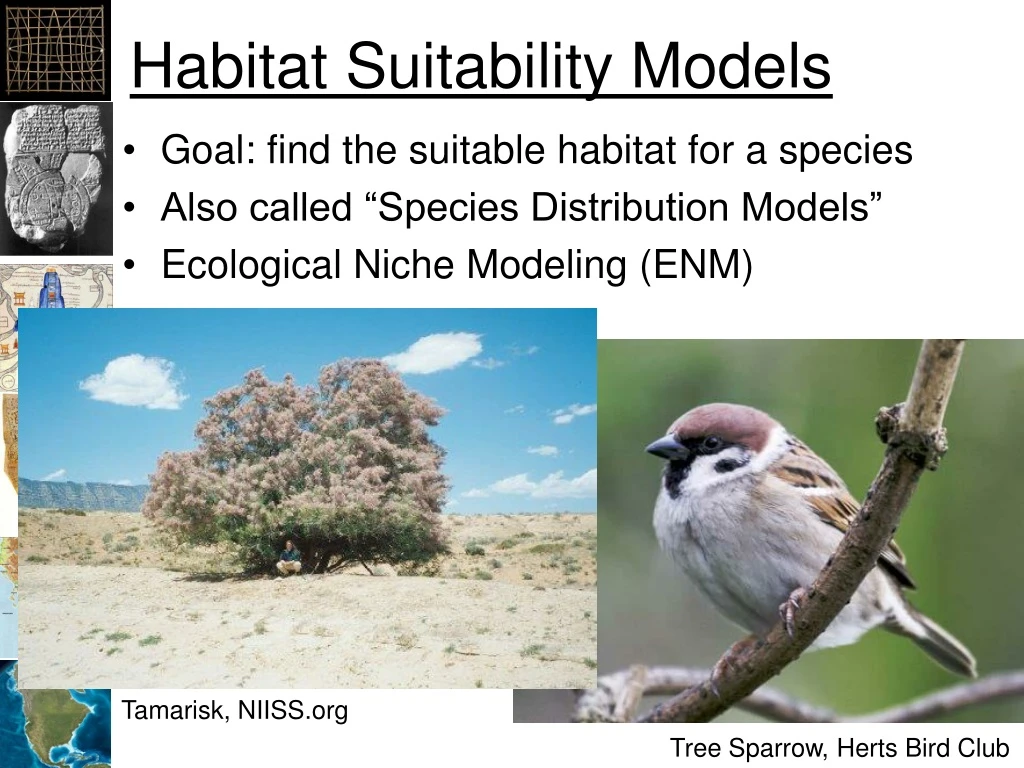
Habitat Suitability Models. Goal: find the suitable habitat for a species Also called “Species Distribution Models” Ecological Niche Modeling (ENM ). Tamarisk, NIISS.org. Tree Sparrow, Herts Bird Club. Species Are Adapted to Particular Habitats. US National Park Service.

E N D
Habitat Suitability Models • Goal: find the suitable habitat for a species • Also called “Species Distribution Models” • Ecological Niche Modeling (ENM) Tamarisk, NIISS.org Tree Sparrow, Herts Bird Club
Species Are Adapted to Particular Habitats US National Park Service
Predicting Habitat Suitability • Predicting potential species distributions at large spatial and temporal extents • Given: • Limited data • Most have unknown uncertainty • Most biased/not randomly sampled • >90% just “occurrences” or “observations” • Lots of species • Climate change and other scenarios
Methods • Density, Abundance: • Continuous response • Linear Reg., GLM, GAMs, BRTs • Presence/Absence: • logit/logistic • What does absence mean? • Presence-Only (occurrences) • What to regress against?
Presence Only • Need to have something to regress against • Obtain background points or pseudo-absences • Sample a portion or all of the sample area • Regress the density of presences vs. the density of the sample area in the environmental space • Regress density of presence against density of predictor values • Jeff Dunk: Point-process problem
From the Theory of Biogeography + 0 - Salinity Environmental Space Population Growth Niche + 0 - Salinity Temperature Temperature Brown, J.H., Lomolino, M.V. 1998, Biogeography: Second Edition. Sinauer Associates, Sinauer Massachusetts
GAM NPMR 2006, MccCune, Non-parametric habitat models with automatic interactions
HSM Are Powerful Tools • Can predict potential habitat for species under changing environmental conditions • Climate, pollution, water, human impacts • Because HSMs are based on environmental data, they do not predict a species distribution. However, they are also called Species Distribution Models (SDMs)
Predicted Distribution of Bigfoot (a) for the present climate and (b) under a possible climate change scenario involving a doubling of atmospheric CO2 levels - Lozier, Predicting the distribution of Sasquatch in western North America: anything goes with ecological niche modelling
HSM Issues clizen.org Human-Modified Environments Isolated Areas North Island, Seychelles PHOTO: AUSTEN JOHNSTON
Early Methods • BioClim • BioMapper • Genetic Algorithm for Rule Set Production (GARP) • Generalized Linear Models (GLM) • Generalized Additive Models (GAMs) • Kernel Methods • Neural Networks
Latest Methods • Multivariate adaptive regression splines (MARS) • MaxEnt – piece-wise regression with Maximum Entropy optimization • Hyper-Envelope Modeling Interface (HEMI 2), Bezier curves • Non-Parametric Multiplicative Regression (NPMR)
Tree Methods • Regression Trees • Boosted Regression Trees • Random Forests
Two Overall Approaches Occurrence/Presence Mechanistic Occurrences “Greenhouse” experiments Correlate Design Model Model Predictor Layers Generate Generate Map
Doug-Fir vs. Temperature Optimal Habitat Poor Habitat
Doug-Fir vs. Temperature Relative Density of Occurrences Mean Annual Temperature in degrees C * 10 Green: histogram of environmental variable values, Red: histogram of occurrences
Doug-Fir vs. Precipitation Optimal Habitat Poor Habitat
Doug-Fir vs. Precipitation Relative Density of Occurrences Annual Precipitation in Millimeters Green: histogram of environmental variable values, Red: histogram of occurrences
Geographical Space Observed Occurrences Realized Niche/Distribution Environmental Space Fundamental Niche/Distribution Model Fitted to Occurrences Adapted from Richard Pearson, Center for Biodiversity and Conservation at the American Museum of Natural History
“Good” Model Douglas-Fir Model with Just Annual Precipitation
“Poor” Model Douglas-Fir Model with Just Annual Precipitation
Modeling Process 100 0 Spreadsheets Occurrences Environmental Layers Temperature Precipitation Modeling Algorithm Model Parameters Habitat Suitability Map Map Generation
ROC Curve • Receiver operating characteristic (ROC) • See: • Wikipedia
Area Under the Curve (AUC) • Area under an ROCcurve • Popular for HSM • Encourages over-fitting
AUC • Advantages • Provides comparable range: • 0.5 – random • 1 – perfect model • Easy to compute • Disadvantages • Does not include number of parameters so encourages over fitting • Increasing the study area increases the AUC value
AIC • Can now be computed for HSMs with ENMTools, Presence/Absence library for R, or BlueSpray • Is this the “best” measure?
Uncertainty in Data • Experts more accurate in correctly identifying species than volunteers • 88% vs. 72% • Volunteers: 28% false negative identifications and 1% false positive identifications • Experts: 12% false negative identifications and <1% false positive identifications • Conspicuous vs. Inconspicuous • Volunteers correctly identified “easy” species 82% of the time vs. 65% for “difficult” species • 62% of false ids for GB were CB
Correcting for Environmental Variability • The previous examples assume a uniform distribution of environmental variation (i.e. same area for each value). • Dividing the number of occurrences by the relative area for each environmental variable value corrects for this.
Doug-Fir vs. Precipitation Relative Density of Occurrences Annual Precipitation in Millimeters Green: histogram of environmental variable values, Red: histogram of occurrences, Blue: Red / Green
Doug-Fir vs. Temperature Relative Density of Occurrences Annual Temperature in degrees C * 10 Green: histogram of environmental variable values, Red: histogram of occurrences, Blue: Red / Green
Spatial Modeling Concerns • Over fitting the data • Are we modeling biological/ecological theory? • What does the model look like? • In environmental space vs. geographic space • Absence points? • What do they mean? • Analysis and representation of uncertainty? • Can we really model the potential distribution of a species from a sub-sample?
Over-fitting The Data? Maxent model for Tamarix in the US: response to temperature when modeled with temperature and precipitation What should the model look like? Maraghni, M., M. Gorai, and M. Neffati. 2010. Seed germination at different temperatures and water stress levels, and seedling emergence from different depths of Ziziphus lotus. South African Journal of Botany 76:453-459.
Maxent Model Parameters • bio12_annual_percip_CONUS, -4.946359908378759, 52.0, 3269.0 • bio1_annual_mean_temp_CONUS, 0.0, -27.0, 255.0 • bio1_annual_mean_temp_CONUS^2, -0.268525818823649, 0.0, 65025.0 • bio12_annual_percip_CONUS*bio1_annual_mean_temp_CONUS, 7.996877654196997, -15579.0, 364506.0 • (681.5<bio12_annual_percip_CONUS), -0.27425992202014554, 0.0, 1.0 • (760.5<bio12_annual_percip_CONUS), -0.0936978541445044, 0.0, 1.0 • (764.5<bio12_annual_percip_CONUS), -0.34195651409710226, 0.0, 1.0 • (663.5<bio12_annual_percip_CONUS), -0.002670474531339423, 0.0, 1.0 • (654.5<bio12_annual_percip_CONUS), -0.06854638847398926, 0.0, 1.0 • (789.5<bio12_annual_percip_CONUS), -0.1911885535421742, 0.0, 1.0 • (415.5<bio12_annual_percip_CONUS), -0.03324755386105751, 0.0, 1.0 • (811.5<bio12_annual_percip_CONUS), -0.5796722427924351, 0.0, 1.0 • (69.5<bio1_annual_mean_temp_CONUS), 0.35186971641045406, 0.0, 1.0 • (433.5<bio12_annual_percip_CONUS), -0.4931182020218725, 0.0, 1.0 • (933.5<bio12_annual_percip_CONUS), -0.6964667980858589, 0.0, 1.0 • (87.5<bio1_annual_mean_temp_CONUS), 0.026976617714580643, 0.0, 1.0 • (41.5<bio1_annual_mean_temp_CONUS), 0.16829480000216024, 0.0, 1.0 • (177.5<bio1_annual_mean_temp_CONUS), -0.10871555671575972, 0.0, 1.0 • (91.5<bio1_annual_mean_temp_CONUS), 0.146912383178006, 0.0, 1.0 • (1034.5<bio12_annual_percip_CONUS), -2.6396398836001156, 0.0, 1.0 • (319.5<bio12_annual_percip_CONUS), -0.061284542503119606, 0.0, 1.0 • (175.5<bio1_annual_mean_temp_CONUS), -0.2618197321200044, 0.0, 1.0 • (233.5<bio1_annual_mean_temp_CONUS), -0.9238257709966757, 0.0, 1.0 • (37.5<bio1_annual_mean_temp_CONUS), 0.3765193693625046, 0.0, 1.0 • (103.5<bio1_annual_mean_temp_CONUS), 0.09930300882047771, 0.0, 1.0 • (301.5<bio12_annual_percip_CONUS), -0.1180307164256701, 0.0, 1.0 • (173.5<bio1_annual_mean_temp_CONUS), -0.10021086459501297, 0.0, 1.0 • (866.5<bio12_annual_percip_CONUS), -0.26959719615289196, 0.0, 1.0 • (180.5<bio1_annual_mean_temp_CONUS), -0.04867293241613234, 0.0, 1.0 • (393.5<bio12_annual_percip_CONUS), -0.11059348100482837, 0.0, 1.0 • (159.5<bio1_annual_mean_temp_CONUS), -0.017616972634255934, 0.0, 1.0 • (36.5<bio1_annual_mean_temp_CONUS), 0.060674971087442194, 0.0, 1.0 • (188.5<bio1_annual_mean_temp_CONUS), -0.03354825843486451, 0.0, 1.0 • (105.5<bio1_annual_mean_temp_CONUS), 0.06125114176950926, 0.0, 1.0 • (153.5<bio1_annual_mean_temp_CONUS), -0.12297221415244217, 0.0, 1.0 • (1001.5<bio12_annual_percip_CONUS), -0.45251593589861716, 0.0, 1.0 • (74.5<bio1_annual_mean_temp_CONUS), 0.026393316564235686, 0.0, 1.0 • (109.5<bio1_annual_mean_temp_CONUS), 0.14526936669793344, 0.0, 1.0 • (105.0<bio12_annual_percip_CONUS), -0.42488171108453276, 0.0, 1.0 • (25.5<bio1_annual_mean_temp_CONUS), 0.003117221628224885, 0.0, 1.0 • (60.5<bio12_annual_percip_CONUS), 0.5069564460069241, 0.0, 1.0 • (231.5<bio12_annual_percip_CONUS), -0.08870602107253492, 0.0, 1.0 • (58.5<bio1_annual_mean_temp_CONUS), -0.23241170568516853, 0.0, 1.0 • (49.5<bio1_annual_mean_temp_CONUS), 0.026096163653731276, 0.0, 1.0 • (845.5<bio12_annual_percip_CONUS), -0.24789751889995176, 0.0, 1.0 • 'bio1_annual_mean_temp_CONUS, -6.9884695411343865, 232.5, 255.0 • (320.5<bio12_annual_percip_CONUS), -0.10845844949785532, 0.0, 1.0 • (121.5<bio1_annual_mean_temp_CONUS), -0.12078290084760739, 0.0, 1.0 • (643.5<bio12_annual_percip_CONUS), -0.18583722923085083, 0.0, 1.0 • (232.5<bio1_annual_mean_temp_CONUS), -0.49532279859757916, 0.0, 1.0 • (77.5<bio12_annual_percip_CONUS), 0.09971599046855084, 0.0, 1.0 • (130.5<bio1_annual_mean_temp_CONUS), -0.01184619743061956, 0.0, 1.0 • (981.5<bio12_annual_percip_CONUS), -0.29393286794072015, 0.0, 1.0 • `bio12_annual_percip_CONUS, 0.023135559662549977, 52.0, 147.5 • 'bio1_annual_mean_temp_CONUS, 1.0069995641400011, 216.5, 255.0 • `bio1_annual_mean_temp_CONUS, 0.9362466512437257, -27.0, 16.5 • (397.5<bio12_annual_percip_CONUS), -0.02296169875555788, 0.0, 1.0 • `bio12_annual_percip_CONUS, 0.14294702222037983, 52.0, 251.5 • (174.5<bio1_annual_mean_temp_CONUS), -0.01232159395283821, 0.0, 1.0 • 'bio1_annual_mean_temp_CONUS, -1.011329703865716, 150.5, 255.0 • `bio12_annual_percip_CONUS, 0.12595056977305263, 52.0, 326.5 • 'bio1_annual_mean_temp_CONUS, -0.6476124017711095, 119.5, 255.0 • 'bio1_annual_mean_temp_CONUS, 1.737841121141096, 219.5, 255.0 • (90.5<bio1_annual_mean_temp_CONUS), 0.012061755141948361, 0.0, 1.0 • `bio12_annual_percip_CONUS, 0.1002190195916142, 52.0, 329.5 • `bio12_annual_percip_CONUS, 0.3321425790853447, 52.0, 146.5 • `bio12_annual_percip_CONUS, -0.3041756531549861, 52.0, 59.0 • (385.5<bio12_annual_percip_CONUS), -0.0014858371668052357, 0.0, 1.0 • (645.5<bio12_annual_percip_CONUS), -0.02553082983087001, 0.0, 1.0 • 'bio12_annual_percip_CONUS, -4.091264412509243, 532.5, 3269.0 • `bio1_annual_mean_temp_CONUS, -0.35523981011398936, -27.0, 111.5 • `bio1_annual_mean_temp_CONUS, -0.21070138315106224, -27.0, 112.5 • `bio1_annual_mean_temp_CONUS, 0.22680342516229093, -27.0, 18.5 • (13.5<bio1_annual_mean_temp_CONUS), -0.04258692136695379, 0.0, 1.0 • `bio1_annual_mean_temp_CONUS, 0.12827234634968193, -27.0, 19.5 • linearPredictorNormalizer, 2.2050375426546283 • densityNormalizer, 1311.2581836276431 • numBackgroundPoints, 10000 • entropy, 8.358957722359722 162 Parameters Maxent model from Tamarix model of western US using precipitation and temperature.
Document Caveats • Assumptions • No errors in the data collection, handling, processing • No software defects • Occurrences represent viable populations in the wild • Density of occurrences correlates with potential habitat • Uncertainties • Field data, environmental layers • 256x256 grid used for 2d histograms
Some Caveats • We are modeling “observations” • Modeling occurrences with some uncertainty • Modeling the realized niche if the data is a complete sample for the environmental space the species currently occupies • Modeling the fundamental niche if B is true and the species is covering it’s full possible range of habitats • Habitat Suitability Modeling • Predicting the potential species distribution
Migration Animations • Jim’s web site • http://tinyurl.com/6krghts • Gray whale model • http://tinyurl.com/4xtmzho • Barn swallows
Oregon Marine Planning Data • Scientific and Technical Advisory Committee (STAC) Review • Materials: • http://oregonocean.info/index.php?option=com_content&view=article&id=480:stac-review-of-oregon-marine-planning-data&catid=15:stay-up-to-date-on-ocean-alternative-energy&Itemid=12
Tree Sparrow Occurrences House Sparrows Eurasian Tree Sparrows Graham, J., C. Jarnevich, N. Young, G. Newman, T. Stohlgren, How will climate change affect the potential distribution of Eurasian Tree Sparrows (Passer montanus)? Current Zoology, 2011.
Tree Sparrow Model - 2050 Graham, J., C. Jarnevich, N. Young, G. Newman, T. Stohlgren, How will climate change affect the potential distribution of Eurasian Tree Sparrows (Passer montanus)? Current Zoology, 2011
Western Larch in NA 2006, MccCune, Non-parametric habitat models with automatic interactions
Doug-Fir vs. Precipitation Douglas-Fir vs. Annual Precipitation
Montane Frogs in Rainforest 2013, Marcio et al., Understanding the mechanisms underlying the distribution of microendemic montane frogs (Brachycephalus spp., Terrarana: Brachycephalidae) in the Brazilian Atlantic Rainforest (a. all records, b. combined with other models)