Download
1 / 63
630 likes | 869 Views
Advanced Suitability Modeling. RESM 575 Spring 2010 Lecture 2. Last time. What is spatial analysis? What is advanced spatial analysis? RESM 575 Lab Geoprocesing Model builder. Today. Overview of papers Advanced suitability modeling Boolean overlay Process models

E N D
Advanced Suitability Modeling RESM 575 Spring 2010 Lecture 2
Last time • What is spatial analysis? • What is advanced spatial analysis? • RESM 575 • Lab • Geoprocesing • Model builder
Today • Overview of papers • Advanced suitability modeling • Boolean overlay • Process models • Index overlay – MCA (Eastman et al. 1995) • Fuzzy logic • Lab: suitability modeling
GIS use • An information database • Coordinating and accessing geographic data • As an analytical tool • Specifying logical and mathematical relationships among map layers • As a decision support tool • For deciding how to act upon the analyses produced (Eastman, et al. 1995)
As an information database • Get nothing more from the system than what went in • May be able to do some neat query with the data • Just a data bank
As an analytical tool • Special geoprocessing tools for creating new information • Knowledge learned from relationships and/or processes • Need to know how to act upon our models
As a decision support tool • Can help us make decisions about multiple and conflicting objectives • Borrows from the decision science or operations research literature • Raster based and vector information processing
GIS modeling and integration • Considerable interest has been focused on the use of GIS as a decision support system. • In decision making we are concerned with the choice between alternatives. • They might be alternative actions, alternative hypotheses about a phenomenon, alternative locations to select or propose, etc.
Integration output map = f (2 or more input maps) • The function, f, takes many different forms, but the relationships expressed by the function are either based on a theoretical understanding of physical and chemical principles, or they are empirical, based on observations of data, or some blend of theory and empiricism (Bonham-Carter, 1994).
Maps Quantitative Integration Attributes of the attribute tables
Steps of map integration • Step 1 • Step 2 • Step 3 Build Spatial Database Data Processing Apply integration models
Boolean operators Most commonly used Process models Integration models Index overlay • Advanced mathematical models • Fuzzy logic • Logistic regression • Dempster-Schafer • Neural Networks • etc
Raster cell values • Cell values represent geographic features • Types of cell values: Binary (0,1) Presence/absence Integers Coded values or whole numbers Floating point Values with decimal places Vector data converted to raster Land use, elevation Slope, aspect
The Raster Calculator • Use with Analysis mask, analysis extent to “clip” rasters • Use to base new raster on existing raster • Convert m to ft Use these buttons • Can also be used to find cells meeting query expressions: • [Slope] > 10% • ([Elevation] > 500) and ([Elevation] < 1000) • Note raster layer names in square brackets [like this] List of raster layers Query Expression window
Map algebra • Raster calculator can also perform map algebra (mathematical functions on raster layers) • Examples: • [Elevation] * 10 • [Grid 1] * [Grid 2] • Log [Grid 1] • Many other ARC/INFO GRID functions – see help for details
NODATA cells • Special cell value • Used to indicate: • No value at location • No data at location (missing) • Data outside study boundary • NODATA is not zero! • Can affect calculations in Spatial Analyst * =
AND = when both corresponding grid cells are nonzero then output is 1, otherwise output is 0 OR = if either of the corresponding grid cells are zero then output is 1, otherwise output is 0 XOR = when one of corresponding grid cells is zero then output is 1, otherwise 0
Practice #1 - Transform int[ingrid] = = [ingrid] >= 5 [ingrid] >1 & [ingrid] <= 6 = ND = no data
Practice #1 – Transform ANSWERS int[ingrid] = = [ingrid] >= 5 [ingrid] >1 & [ingrid] <= 6 = ND = no data
Practice #2 - Overlay and = or = xor = ND = no data
AND = when both corresponding grid cells are nonzero then output is 1, otherwise output is 0 OR = if either of the corresponding grid cells are zero then output is 1, otherwise output is 0 XOR = when one of corresponding grid cells is zero then output is 1, otherwise 0 Practice #2 – Overlay ANSWERS and = or = xor = ND = no data
Limitations with boolean operators • Although, Boolean operation is an easy and fast model to run, there are some problems in its execution routine. The results can be binary. • In a binary map only 2 situations are possible, each location is either satisfactory or not.
Notes • Integration by Boolean operators is a very extreme form of decision making. • For example if logical AND (the intersection operator), is applied to combine the criteria a location must meet every criterion for it to be included in the final decision set. • If even a single criterion fails to be met, the location will be excluded in the final binary result map. • “Risk adverse”, “Conservative”
Process modeling • Integration in process modeling in GIS is based on already suggested methodology or formula(s).
Example 1 of a process model Model for snow melt in densely forested areas MELT = (0.19T + .17D) Where M is the melt rate in cm/day T is temperature in Celsius D is dewpoint temperature We could clearly produce a snow melt rate map (M). To do so would require multiplying the temperature raster by 0.19, the dewpoint raster by 0.17 and adding the two results. * Dunne, T., and Leopold, L.B., (1978) Water in Environmental Planning, (W.H. Freeman and Co.: San Francisco)
Example 2 of process model By preparing the data as recommended and integrating them in a GIS, simulation or predictive map(s) representing the phenomena can be generated. Such methodologies and processes are usually recommended by researchers.
Multiple criteria in decision making • Usually several criteria will need to be evaluated all together in order to meet a specific objective.
Suitability models An interpretation of data with respect to its suitability for an activity Typically used to locate something (no definable units to compare) Results in a numeric measure of suitability Used when the problem is complex or important Suitability scores can be subjective or quantitative
Suitability models If designed properly, the model results in potential locations being identified and assigned a relative suitability score for the activity. (the best sites have the highest suitability scores) Helps you systematically organize your criteria and decisions More “liberal” mapping of areas compared to boolean
Compared to boolean overlay… • Index Overlay model has more flexibility and ability for priority indication on spatial units of factormaps. • Index overlay method is a simple and commonly used method for GIS layer integration to generate suitability, potential , risk maps,…etc.
Building suitability models, steps Define the problem or goal Decide on evaluation criteria Normalize and create utility scales Define weights for criteria Calculate a ranking model result Evaluate result
Options for reclassifying Many different methods are proposed for standardization for example: • Reclassification (converting continuous variables to ordinal scale) • If all factors are numerical and normally distributed, calculating normal zscore • Reclassification to fuzzy membership values • Applying “normalizing” calculations such as: using minimum and maximum
Premise • We rarely have perfect information • We rarely have error free data • Leads to uncertainty in decision making rules
Uncertainty in using GIS for suitability modeling • Which parameters, attributes or thresholds should we use in our index overlays? • What is a gentle slope? • If less than 5% is gentle, what about 5.001% slope? Is it not gentle? • No distinct or sharp boundaries – it is fuzzy!
Fuzziness • Refers to vagueness and uncertainty, in particular to the vagueness related to human language and thinking • “ the set of tall people” • “all people living close to my home” • “all areas that are suitable for corn” • Provides a way to obtain conclusions from vague, ambiguous or imprecise information. It imitates the human reasoning process of working with non precise data.
Crisp sets versus fuzzy sets Fuzzy sets Membership function UA: X -> [0, 1] where UA(X) is the membership value of x in A Crisp sets Characteristic function XA: X -> {0,1} where 1 iff X є A XA(X) = 0 iff X є A {
Example of crisp sets versus fuzzy sets • Height of three adults: A is 178cm, B is 166cm, and C is 181cm Characteristic Function Crisp set short under 170cm average 170 to 180cm tall over 180cm short tall ave 1 B C A 0 height 170 180 short tall ave 0 1 0 A B C 1 0 0 0 0 1
Example of crisp sets versus fuzzy sets • Height of same three adults: A is 178cm, B is 166cm, and C is 181cm short tall ave 1 .75 Membership Function .5 .25 B A C 0 height 170 180 short tall ave 0 .4 .6 A B C .8 .2 0 0 .3 .7
Steps of map integration with fuzzy logic Selecting a fuzzy membership function Assigning fuzzy membership values to classes (regions) of each map based on the selected function Calculating (integrating) overall fuzzy membership value of maps based on a fuzzy logic combination operator(s)
Choice of membership function • The grade of membership should be 1 at the center of the set • The membership function should fall off in an appropriate way from the center through the boundary • The point with membership grade .5 (crossover point) is at the boundary of the crisp set
Choice of membership function • The membership function depends on the application • EX: moderate elevation may be defined much differently in West Virginia versus moderate elevation in Colorado • There are linear and sinusoidal membership functions, I will focus on linear in the example which follows Ave height 1 B A C 0 170 180