Download
1 / 31
330 likes | 479 Views
Presented by Joseph K. Berry W. M. Keck Scholar, Department of Geography, University of Denver. Introduction to GIS Modeling Week 3 — Reclassifying and Overlaying Maps GEOG 3110 –University of Denver. …but we didn’t finish last week’s material!!!. Suitability Modeling Logic

E N D
Presented byJoseph K. Berry W. M. Keck Scholar, Department of Geography, University of Denver Introduction to GIS ModelingWeek 3 — Reclassifying and Overlaying Maps GEOG 3110 –University of Denver …but we didn’t finish last week’s material!!! Suitability Modeling Logic Reclassifying Maps (position, initial value, size, shape and contiguity) Overlaying Maps (point-by-point, region-wide and map-wide)
Display Settings for Grid-based Maps <Exercise 3 Question #1> Let’s look at some example displays in the Bighorn.rgs data base… (Berry)
Reclassify and Overlay Operations <Exercise 3 Question #2> <Exercise 3 Question #3> Covertype (Input map) Size (Command) SIZE Covertype FOR Covertype_size …make sure your map display is “appropriate” –not simply the default Covertype_size (Output map) (Berry)
Evaluating Habitat Suitability Generating maps of animal habitat… Manual Map Overlay (Binary) Ranking Overlay (Binary Sum) Rating Overlay (Rating Average) (digital slide show Hugag) <Exercise 3 Question #4> Assumptions– Hugags like… gentle slopes, southerly aspects, and lower elevations (See Beyond Mapping III online book, “Topic 23” for more information) (Berry)
Conveying Suitability Model Logic gentle slopes Elevation Slope Slope Preference Bad 1 to 9 Good Reclassify (Times 1) southerly aspects Elevation Aspect Aspect Preference Bad 1 to 9 Good Habitat Rating Bad 1 to 9 Good (1) Reclassify Overlay lower elevations (1) Elevation Elevation Preference Bad 1 to 9 Good Reclassify Habitat Rating 0= No-go 1 to 9 Good Overlay Algorithm Calibrate Weight Base Maps Derived Maps Interpreted Maps Solution Map Fact Judgment Covertype Water Mask 0= No, 1= Yes Reclassify Constraint Map Rows Model Criteria Columns Analysis Levels Lines Processing Steps (Commands) …while Reclassifyand Overlaycommands are not very exciting, they are some of the most frequently used operations (See Beyond Mapping III online book, “Topic 22” for more information) (Berry)
Extending Model Criteria (Times 10) (1) (1) forests Forests Forest Proximity Forest Preference Bad 1 to 9 Good (10) • Hugags are 10 times more concerned with slope, forest and water criteriathan aspect and elevation water Water Water Proximity Water Preference Bad 1 to 9 Good (10) gentle slopes Rows Model Criteria Columns Analysis Levels Elevation Slope Slope Preference Bad 1 to 9 Good southerly aspects Elevation Aspect Aspect Preference Bad 1 to 9 Good Habitat Rating Bad 1 to 9 Good Lines Processing Steps (Commands) lower elevations Additional criteria can be added… Elevation Elevation Preference Bad 1 to 9 Good • Hugags would prefer to be in/near forested areas • Hugags would prefer to be near water (Berry)
Optional Questions Using PowerPoint as a “graphics package” 3-1) Flowchart of Binary Habitat Model 3-2) “Simply” and “Completely” Crosstab Tables 3-3)Average Suitability Rating for eachCovertype parcel 3-4)Average and Coefficient of Variation maps for the 200 foot contour polygons of Elevation (statistical model) 3-5)Average Wildfire Fuel Loading index for each management District (mathematical model) (Berry)
Creating a Flowchart (using PowerPoint) Enter map title Under the Home tab, 1) use the Rectangle drawing tool to create and size a box to represent a map in the flowchart and 2) use the Textbox drawing tool to enter the map name in the Rectangle. Selectboth and use Format Groupto group the two objects. 2 1 Enter map title Enter other map title Copy and Paste the Rectangle to form other maps. Use theLinedrawing tool to connect the boxes. Use the Textbox drawing tool to enter the command, rotate and place over the Line. Slope Enter yet another map title Repeatthe process to add additional maps (boxes) and processing steps (lines) to complete the flowchart containing the logic of the GIS model. There are a lot of other things you can do to make the graphic a bit more unique, such as borders, transparency, shadowing and animation (viewed as a slide show). Also, keep in mind that Format Align can be used to align multiple graphic objects if things get out of whack. (Berry)
Compound Graphic (Campground model results) Campground Suitability Use SnagIt to capture one of the graphic elements, such as the S_Pref map then Paste and Size at the appropriate location on the “canvas” (white background shape). Repeat for all of the other graphic elements. Use the Text Box tool to embed text as appropriate. Group the figure elements in logical groupings and then use the Custom Animation tool to control their sequencing for display if you intend to present as a PowerPoint slide deck. (Berry)
Big Picture of Map Analysis and Modeling Statistician’s Perspective: Nanotechnology GEOTECHNOLOGY Biotechnology Basic Descriptive Statistics Basic Classification Map Comparison Unique Map Statistics Surface Modeling Advanced Classification Predictive Statistics Global Positioning System GEOGRAPHIC INFORMATION SYSTEMS Remote Sensing ANALYSIS andMODELING (Grid-based) Mapping and Geo-query (Vector-based) SPATIAL ANALYSIS (Geographic Relationships) SPATIAL STATISTICS (Numeric Relationships) GISer’s Perspectives Week 3 Week 8 Reclassify and Overlay Distance and Neighbors Surface Modeling Spatial Data Mining Basic GridMath & Map Algebra Advanced GridMath Map Calculus Map Geometry Plane Geometry Connectivity Solid Geometry Connectivity Unique Map Analytics Week 4 Week 5 Week 9 Mathematician’s Perspective: GIS Modeling Weeks 6 and 7 Future Directions Week 10 Math/Stat Perspectives (SpatialSTEM) See Topic 30, Beyond Mapping III (Berry)
Grid-Based Map Analysis • Spatial analysisinvestigates the “contextual” relationships in mapped data… • Reclassify— reassigning map values (position; value; size, shape; contiguity) • Overlay— map overlay (point-by-point; region-wide; map-wide) • Distance— proximity and connectivity (movement; optimal paths; visibility) • Neighbors— ”roving windows” (slope/aspect; diversity; anomaly) Weeks 3,4,5 Spatial statistics • Surface modelingmaps the spatial distribution and pattern of point data… • Map Generalization— characterizes spatial trends (e.g., titled plane) • Spatial Interpolation— deriving spatial distributions (e.g., IDW, Krig) • Other— roving window/facets (e.g., density surface; tessellation) • Data mininginvestigates the “numerical” relationships in mapped data… • Descriptive— aggregate statistics (e.g., average/stdev, similarity, clustering) • Predictive— relationships among maps (e.g., regression) • Prescriptive— appropriate actions (e.g., optimization) Weeks,8,9 (Berry)
An Analytic Framework for GIS Modeling …recall Map Analysis organization and evolution discussion from Week 1 class presentation/reading (GIS Modeling Framework paper) Reclassify operationsinvolve reassigning map values to reflect new information about existing map features (Berry)
Reclassifying Maps (Berry)
Reclassifying Maps <Homework Question #2> CLUMP -- Assigns new values to contiguous groups of cells within each map category. CONFIGURE -- Assigns new values characterizing the shape of the area associated with each category. RENUMBER -- Assigns new values to the categories of a map. SIZE -- Assigns new values according to the size of the area associated with each map category. SLICE -- Assigns new values by dividing the range of values on a map into specified intervals (contouring). Contiguity Shape The most frequently used map analysis operation …and one of the most dangerous!!! Initial Value Size Initial Value (Berry)
…any real number from -3.4E38 to + 3.4E38can be assigned to any existing value on a map …often integer values are assigned based on user reasoning (as in this example) Note: PMAP_NULL is a special value that can be assigned indicating “no data” and the grid location will be ignored in processing and display …context Help provides information on function and use of operations <more info in the MapCalc Manual> Renumber Operation Renumber— assigns new values to the categories of a map. RENUMBER Elevation ASSIGNING 1 TO 500 THRU 1800 ASSIGNING 0 TO 1800 THRU 2500 FOR E_Pref (Berry)
…Map Range = Max_Value – Min_Value = 2500 – 500= 2000 feet …Contour Interval = Map Range / # ranges = 2000 / 20 = 100 feet SLICE Elevation into 20 FOR Relief_100ft …a user can specify the minimum and maximum values of the range– SLICE Elevation INTO 20 FROM 1000 THRU 1200 ZeroFill FOR Relief_10ft …Slice <mapName>is often used to collapse a map with a large set of map values to just a few intervals for a quick view of the pattern of the spatial data distribution Slice Operation Slice— assigns new values by dividing the range of values on a map into specified intervals (“Equal Ranges” contouring) (Berry)
…to calculate the actual area of each map region multiply the size map times the area per grid cell– 10,000 m2 or 1 ha in this case …to calculate the size/area of each occurrence you must first Clump the map “regions”, then use the Size command Size Operation Size— assigns new values according to the size of the area associated with each map category. …the Size operation assigns the number of cells comprising each map region (category/value) …in this instance there are three map regions (Open Water= 1, Meadow= 2, Forest= 3)– note that Water occurs at two different places. SIZE Covertype FOR Coverype_size (Berry)
“At” identifies how far to reach in defining clumps “Orthogonally” reaches horizontally and vertically only; “Diagonally” includes off angles Clump Operation Clump— assigns new values to contiguous groups of cells within each map category. …a map “category” identifies all locations with the same characteristic or condition– e.g., Open Water, Meadow, Forest …a “clump” is a contiguous group (individual spatial instance of a map “category”)–e.g., five cover type clumps with two instances of Open Water CLUMP Covertype AT 1 DIAGONALLY FOR Coverype_clumps (Berry)
Configure Operation Configure— assigns new values characterizing the shape and integrity of the area associated with each map category. Boundary Configuration Convexity is the ratio of the Edge to the Area (Size) and normalized to that of a circle of the same area CONFIGURE Covertype Edges FOR Covertype_edges Edge cells Spatial Integrity Euler = (# Holes) – (1-#Fragments) (Berry)
Some Reclassifying Things to Keep in Mind The Covertype map contains Nominal data that is Discretely (Choropleth) distributed in geographic space. As such, it is best displayed in 2D using cells (Grid) and with layer mesh on as the stored values do not form gradients in either numerical or geographic space. The Size command assigns new values according to the size of the area (# of cells) associated with each map category. In this instance the input map is Covertype (Nominal/Discrete data) and the output map is Covertype_size (Ratio/Discrete data). The size algorithm “counts” the number of cells for each map category (stored map value). Size works on Nominal data (Categorical) but usually is not appropriate for ratio data as far to many values (decimal places); results in most of the map being assigned the cell size value of 1 because elevation values with decimal points rarely are the same. For example, sizing the Elevation map… …identifies that “one cell in size” elevation values occur in 64% of the map area (384/1= 384 times; each value is unique). “Three cells in size” areas occur in 2.88% of the analysis window (18/3= 6 times; six sets of the same value). (Berry)
An Analytic Framework for GIS Modeling …recall Map Analysis organization and evolution discussion from Week 1 class presentation/reading (GIS Modeling Framework paper) Overlay operationsinvolve characterizing the spatial coincidence of mapped data (Berry)
Overlaying Maps (accessing the data) Overlaying mapsinvolves one of four basic techniques for accessing/organizing geo-registered data for analysis— (Tomlin’s organizational framework) Local Focal Zonal Global Template Map Entire Area Map1 Map1 Map1 Map1 Map2 Map2 Map2 Map2 “Spearing” “Lacing” “Plunging” “Funneling” …collects data on a cell-by-cell basis and reports a single value on a cell-by-cell basis …collects data on a neighborhood basis and reports a single value on a cell-by-cell basis …collects data on a region-wide basis and reports summary on a region-wide basis …collects data on a map-wide basis and reports results on a map-wide or cell-by-cell basis (Berry)
Overlaying Maps <Homework Question #3> Region- wide COMPOSITE -- Creates a map summarizing values from one map which coincide with the categories of another. CALCULATE and COMPUTE -- Creates a map as the mathematical or statistical function of two or more maps. COVER -- Creates a new map where nonzero values of the top map replace the values on the previous (bottom) map, or stack of maps. CROSSTAB -- Generates a spatial coincidence table of two maps. INTERSECT -- Creates a map that assigns new values to pair-wise combinations of values on two maps. Point-by- Point …true “map-ematics” Point-by- Point Point-by- Point Point-by- Point …Map-wide overlay involves spatial statistics (spatial data mining) (Berry)
Compute/Calculate Operation Compute/Calculate— creates a new map as the mathematical function of two or more maps. All of the basic mathematical operations on a typical pocket calculator can be performed on grid maps… …including Add, Subtract, Multiply, Divide, Exponentiation, Square, Square Root, Max, Min, And, Or, & Trig functions …other math operations? CALCULATE ((Covertype * 10) + Water) FOR Covertype_Water COMPUTE Covertype TIMES 10 Plus Water FOR Coverype_Water …in this example one map is multiplied by 10 then added to another map, thereby creating a 2-digit code indicating the first map’s categories as the tens digit followed by the second map’s categories as the one’s digit (Berry)
Crosstab Operation Crosstab— generates a spatial coincidence table of two maps. …the maps are compared “cell-by-cell” and the number of joint occurrences between the map categories are summarized in a table Map1 = Districts Optional Question 3-2 Map2 = Covertype CROSSTAB Districts WITH Covertype Simply TO Newtextfile.txt • In this example there are… • 58 cells classified as District 1 on the Districts map • 82 cells classified as Open Water on the Covertype map • 58 cells identified as having the joint condition of District 1 and Open Water representing 9.28 percent of the entire map area. • Note: all of the District 1 cells are in Open Water (Berry)
Intersect Operation Intersect— creates a map that assigns new values to pair-wise combinations of values on two maps. Map 1 = Districts The maps are compared “cell-by-cell” and a user specified number is assigned to designated category combinations… …“zerofill” assigns 0 to all combinations that are not specified … “oldfill” retains 1st map values for non-specified combinations Map 2 = Covertype INTERSECT Districts WITH Covertype ASSIGN 1 to 1, 1 Zerofill FOR Districts1_Cover1 …if “completely” is specified all combinations are automatically identified using unique sequential numbering for map values Note: Intersect is similar to geo-query operations in desktop mapping packages by identifying all locations having specified category (map-value) combinations (Berry)
Cover Operation Cover— creates a new map where the non-zero values of the top map replace the values on the previous (bottom) map, or stack of maps. …the maps are compared “cell-by-cell” and the value in the top-most cell replaces the previous values unless that value is zero, then the top most non-zero value in the map stack is retained Water Water 4 4 0 4 Covertype Cover 1 3 1 “Zero” is treated as transparentas maps are staked; non-zero values treated as opaque (0,3 3) (4,1 4) COVER Covertype WITH Water IGNORE 0 FOR Districts1_Cover1 …in the example coincidence 4,1 4 because 4 is non-zero and replaces what is beneath it …0,3 3 because zero is ignored and does not replace the previous value in the map stack (Berry)
Composite Operation Composite— creates a map summarizing values from one map that coincide with the categories (termed regions) identified on another map …the regions identified by category values on one map serve as cookie-cutter shapes (Template map) for summarizing data contained on another map (Data map) Template Map “Cookie-cutter” Data Map COMPOSITE Districts WITH Slope Average IGNORE PMAP_NULL FOR Districts_avgSlope …data summary procedures include Average, Standard deviation, Coefficient of variation, Total, Maximum, Minimum, Median Majority, Minority, Diversity, Deviation and Proportion (Berry)
Thematic Mapping (Average elevation by district) Worst “Thematic Mapping” (Discrete Spatial Object) Average Elevation of Districts 500 1539 2176 Best (0) (39) (9) 653 1099 …include Coffvar in Thematic Mapping results (29) (21) 1779 (9) 1080 (24) (Berry)
Map Accuracy (Error Propagation– simple overlay) P(x,y) P(x) Topological Overlay Joint Probability P(x,y) = P(x) * P(y) Intersect Polygons Spatial Table Attribute Table Join Data P(y) …evaluated cell-by-cell Coincidence Search 100% certain everywhere in the derived polygon? Believable? Soil Type (digital slide show Honest) Vector Raster Forest Type Joint Probability— likelihood of two conditions occurring together… (See Beyond Mapping II, “Topic 4, “Toward and Honest GIS”) (Berry)