Download

1 / 106
1.21k likes | 1.65k Views
6-1 Introduction To Empirical Models. 6-1 Introduction To Empirical Models. Based on the scatter diagram, it is probably reasonable to assume that the mean of the random variable Y is related to x by the following straight-line relationship:.

E N D
6-1 Introduction To Empirical Models Based on the scatter diagram, it is probably reasonable to assume that the mean of the random variable Y is related to x by the following straight-line relationship: where the slope and intercept of the line are called regression coefficients. The simple linear regression model is given by where is the random error term.
6-1 Introduction To Empirical Models We think of the regression model as an empirical model. Suppose that the mean and variance of are 0 and 2, respectively, then The variance of Y given x is
6-1 Introduction To Empirical Models • The true regression model is a line of mean values: • where 1 can be interpreted as the change in the mean of Y for a unit change in x. • Also, the variability of Y at a particular value of x is determined by the error variance, 2. • This implies there is a distribution of Y-values at each x and that the variance of this distribution is the same at each x.
6-1 Introduction To Empirical Models A Multiple Linear Regression Model: where = the intercept of the plane , = partial regression coefficients
6-2 Simple Linear Regression 6-2.1 Least Squares Estimation • The case of simple linear regression considers a single regressoror predictorx and a dependent or response variableY. • The expected value of Y at each level of x is a random variable: • We assume that each observation, Y, can be described by the model
6-2 Simple Linear Regression 6-2.1 Least Squares Estimation • Suppose that we have n pairs of observations (x1, y1), (x2, y2), …, (xn, yn). • The method of least squares is used to estimate the parameters, 0 and 1 by minimizing the sum of the squares of the vertical deviations in Figure 6-6.
6-2 Simple Linear Regression 6-2.1 Least Squares Estimation • Using Equation 6-8, the n observations in the sample can be expressed as • The sum of the squares of the deviations of the observations from the true regression line is
6-2 Simple Linear Regression 6-2.1 Least Squares Estimation
6-2 Simple Linear Regression 6-2.1 Least Squares Estimation
6-2 Simple Linear Regression 6-2.1 Least Squares Estimation
6-2 Simple Linear Regression 6-2.1 Least Squares Estimation
6-2 Simple Linear Regression 6-2.1 Least Squares Estimation
6-2 Simple Linear Regression 6-2.1 Least Squares Estimation
6-2 Simple Linear Regression 6-2.1 Least Squares Estimation
6-2 Simple Linear Regression 6-2.1 Least Squares Estimation
6-2 Simple Linear Regression Sums of Squares and Cross-products Matrix The Sums of squares and cross-products matrix is a convenient way to summarize the quantities needed to do the hand calculations in regression. It also plays a key role in the internal calculations of the computer. It is outputed from PROC REG and PROC GLM if the XPX option is included on the model statement. The elements are X’X
6-2 Simple Linear Regression 6-2.1 Least Squares Estimation
6-2 Simple Linear Regression Regression Assumptions and Model Properties
6-2 Simple Linear Regression Regression Assumptions and Model Properties
6-2 Simple Linear Regression Regression and Analysis of Variance
6-2 Simple Linear Regression Regression and Analysis of Variance
6-2 Simple Linear Regression Example 6-1 OPTIONS NOOVP NODATE NONUMBER LS=80; DATA ex61; INPUT salt area @@; LABEL salt='Salt Conc' area='Roadway area'; CARDS; 3.8 0.19 5.9 0.15 14.1 0.57 10.4 0.4 14.6 0.7 14.5 0.67 15.1 0.63 11.9 0.47 15.5 0.75 9.3 0.6 15.6 0.78 20.8 0.81 14.6 0.78 16.6 0.69 25.6 1.3 20.9 1.05 29.9 1.52 19.6 1.06 31.3 1.74 32.7 1.62 PROC REG; MODEL salt=area/xpx r; PLOT salt*area; /* Scatter Plot*/ RUN; QUIT;
6-2 Simple Linear Regression Linear Regression of SALT vs AREA The REG Procedure Model: MODEL1 Model Crossproducts X'X X'Y Y'Y Variable Label Intercept area salt Intercept Intercept 20 16.48 342.7 area Roadway area 16.48 17.2502 346.793 salt Salt Conc 342.7 346.793 7060.03 ----------------------------------------------------------------------------------------- Linear Regression of SALT vs AREA The REG Procedure Model: MODEL1 Dependent Variable: salt SaltConc Number of Observations Read 20 Number of Observations Used 20 ----------------------------------------------------------------------------------------- Analysis of Variance Sum of Mean Source DF Squares Square F Value Pr > F Model 1 1130.14924 1130.14924 352.46 <.0001 Error 18 57.71626 3.20646 Corrected Total 19 1187.86550 Root MSE 1.79066 R-Square 0.9514 Dependent Mean 17.13500 Adj R-Sq 0.9487 CoeffVar 10.45030 Parameter Estimates Parameter Standard Variable Label DF Estimate Error t Value Pr> |t| Intercept Intercept1 2.67655 0.86800 3.08 0.0064 area Roadway area 1 17.54667 0.93463 18.77 <.0001
6-2 Simple Linear Regression SAS 시스템 The REG Procedure Model: MODEL1 Dependent Variable: salt SaltConc Output Statistics Dependent Predicted Std Error Std Error Student Cook's Obs Variable Value Mean Predict Residual ResidualResidual -2-1 0 1 2 D 1 3.8000 6.0104 0.7152 -2.2104 1.642 -1.346 | **| | 0.172 2 5.9000 5.3085 0.7464 0.5915 1.628 0.363 | | | 0.014 3 14.1000 12.6781 0.4655 1.4219 1.729 0.822 | |* | 0.025 4 10.4000 9.6952 0.5633 0.7048 1.700 0.415 | | | 0.009 5 14.6000 14.9592 0.4168 -0.3592 1.741 -0.206 | | | 0.001 6 14.5000 14.4328 0.4255 0.0672 1.739 0.0386 | | | 0.000 7 15.1000 13.7309 0.4395 1.3691 1.736 0.789 | |* | 0.020 8 11.9000 10.9235 0.5194 0.9765 1.714 0.570 | |* | 0.015 9 15.5000 15.8365 0.4063 -0.3365 1.744 -0.193 | | | 0.001 10 9.3000 13.2045 0.4518 -3.9045 1.733 -2.253 | ****| | 0.173 11 15.6000 16.3629 0.4025 -0.7629 1.745 -0.437 | | | 0.005 12 20.8000 16.8893 0.4006 3.9107 1.745 2.241 | |**** | 0.132 13 14.6000 16.3629 0.4025 -1.7629 1.745 -1.010 | **| | 0.027 14 16.6000 14.7837 0.4195 1.8163 1.741 1.043 | |** | 0.032 15 25.6000 25.4872 0.5985 0.1128 1.688 0.0668 | | | 0.000 16 20.9000 21.1005 0.4527 -0.2005 1.732 -0.116 | | | 0.000 17 29.9000 29.3475 0.7639 0.5525 1.620 0.341 | | | 0.013 18 19.6000 21.2760 0.4571 -1.6760 1.731 -0.968 | *| | 0.033 19 31.3000 33.2077 0.9451 -1.9077 1.521 -1.254 | **| | 0.304 20 32.7000 31.1021 0.8449 1.5979 1.579 1.012 | |** | 0.147 Sum of Residuals 0 Sum of Squared Residuals 57.71626 Predicted Residual SS (PRESS) 70.97373
6-2 Simple Linear Regression 6-2.2 Testing Hypothesis in Simple Linear Regression Use of t-Tests Suppose we wish to test An appropriate test statistic would be
6-2 Simple Linear Regression 6-2.2 Testing Hypothesis in Simple Linear Regression Use of t-Tests We would reject the null hypothesis if
6-2 Simple Linear Regression 6-2.2 Testing Hypothesis in Simple Linear Regression Use of t-Tests Suppose we wish to test An appropriate test statistic would be
6-2 Simple Linear Regression 6-2.2 Testing Hypothesis in Simple Linear Regression Use of t-Tests We would reject the null hypothesis if
6-2 Simple Linear Regression 6-2.2 Testing Hypothesis in Simple Linear Regression Use of t-Tests An important special case of the hypotheses of Equation 6-23 is These hypotheses relate to the significance of regression. Failure to reject H0 is equivalent to concluding that there is no linear relationship between x and Y.
6-2 Simple Linear Regression 6-2.2 Testing Hypothesis in Simple Linear Regression Use of t-Tests
6-2 Simple Linear Regression 6-2.2 Testing Hypothesis in Simple Linear Regression Use of t-Tests
6-2 Simple Linear Regression The Analysis of Variance Approach
6-2 Simple Linear Regression 6-2.2 Testing Hypothesis in Simple Linear Regression The Analysis of Variance Approach
6-2 Simple Linear Regression 6-2.3 Confidence Intervals in Simple Linear Regression
6-2 Simple Linear Regression 6-2.3 Confidence Intervals in Simple Linear Regression
6-2 Simple Linear Regression 6-2.4 Prediction of Future Observations
6-2 Simple Linear Regression 6-2.4 Prediction of Future Observations
6-2 Simple Linear Regression 6-2.5 Checking Model Adequacy • Fitting a regression model requires several assumptions. • Errors are uncorrelated random variables with mean zero; • Errors have constant variance; and, • Errors be normally distributed. • The analyst should always consider the validity of these assumptions to be doubtful and conduct analyses to examine the adequacy of the model
6-2 Simple Linear Regression 6-2.5 Checking Model Adequacy • The residuals from a regression model are ei = yi - ŷi , where yiis an actual observation and ŷi is the corresponding fitted value from the regression model. • Analysis of the residuals is frequently helpful in checking the assumption that the errors are approximately normally distributed with constant variance, and in determining whether additional terms in the model would be useful.
6-2 Simple Linear Regression 6-2.5 Checking Model Adequacy • As an approximate check of normality, construct a frequency histogram or anormal probability plot of residuals. • Standardize the residuals by computing , i = 1, 2, …, n. If the errors are normally distributed, approximately 95% of the standardized residuals should fall in the interval (.
6-2 Simple Linear Regression 6-2.5 Checking Model Adequacy • Plot the residuals (1) in time sequence (if known), (2) against the , and (3) against the independent variable . ,
6-2 Simple Linear Regression 6-2.5 Checking Model Adequacy