Download
1 / 29
330 likes | 560 Views
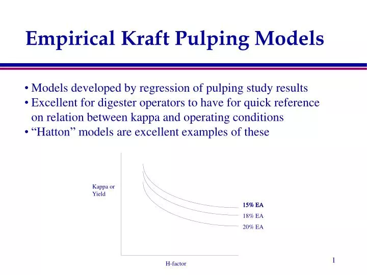
Kappa or Yield. 15% EA. 15% EA. 15% EA. 18% EA. 20% EA. H-factor. Empirical Kraft Pulping Models. Models developed by regression of pulping study results Excellent for digester operators to have for quick reference on relation between kappa and operating conditions

E N D
Kappa orYield 15% EA 15% EA 15% EA 18% EA 20% EA H-factor Empirical Kraft Pulping Models • Models developed by regression of pulping study results • Excellent for digester operators to have for quick reference on relation between kappa and operating conditions • “Hatton” models are excellent examples of these
Emperical Kraft Pulping Models Hatton Equation Kappa (or yield) = -(log(H)*EAn) ,, and n are parameters that must be fit to the data. Values of ,, and n for kappa prediction are shown in the table below. Warning: These are empirical equations and apply only over the specified kappa range. Extrapolation out of this range is dangerous!
Delignification Kinetics ModelsH Factor Model • Uses only bulk delignification kinetics k = Function of [HS-] and [OH-] R = T [=] °K
Delignification Kinetics ModelsH Factor Model k0 is such that H(1 hr, 373°K) = 1 Relative reaction rate
Delignification Kinetics ModelsH Factor Model • Provides mills with the ability to handle common disturbance such as inconsistent digester heating and cooking time variation.
170 900 700 130 Relative Reaction Rate 500 H factor equal to area under this curve Temperature °C 300 90 100 1 2 Hours from Start Delignification Kinetics ModelsH Factor/Temperature
Delignification Kinetics ModelsKerr model ~ 1970 • H factor to handle temperature • 1st order in [OH-] • Bulk delignification kinetics w/out [HS-] dependence
Delignification Kinetics ModelsKerr model ~ 1970 Integrated form: H-Factor Functional relationship between L and [OH-]
Delignification Kinetics ModelsKerr model ~ 1970 Slopes of lines are not a function of EA charge
Delignification Kinetics ModelsKerr model ~ 1970 Model can handle effect of main disturbances on pulping kinetics • Variations in temperature profile • Steam demand • Digester scheduling • Reaction exotherms • Variations in alkali concentration • White liquor variability • Differential consumption of alkali in initial delignification • Often caused by use of older, degraded chips • Good kinetic model for control
Delignification Kinetics ModelsGustafson model • Divide lignin into 3 phases, each with their own kinetics • 1 lignin, 3 kinetics • Transition from one kinetics to another at a given lignin content that is set by the user. For softwood: Initial to bulk ~ 22.5% on wood Bulk to residual ~ 2.2% on wood
Delignification Kinetics ModelsGustafson model • Initial • dL/dt = k1L • E ≈ 9,500 cal/mole • Bulk • dL/dt = (k2[OH-] + k3[OH-]0.5[HS-]0.4)L • E ≈ 30,000 cal/mole • Residual • dL/dt = k4[OH-]0.7L • E ≈ 21,000 cal/mole
Delignification Kinetics ModelsGustafson model Another model was formulated that was of the type dL/dt = K(L-Lf) Where Lf = floor lignin level – set @ 0.5% on wood • Did not result in any better prediction of pulping behavior
Delignification Kinetics ModelsPurdue Model 2 types of lignin: • High reactivity • Low reactivity Assumed to react simultaneously Lf assumed to be zero
Delignification Kinetics ModelsPurdue Model Potential difficulties • High reactivity lignin (initial lignin) dependent on [OH-] and [HS-] • No residual lignin kinetics
Delignification Kinetics ModelsAndersson, 2003 • 3 types of lignin: • Fast • Medium • slow Assumed to react simultaneously, like Purdue model 1 10 total lignin Lignin [%ow] 0 10 L3 lignin L1 lignin L2 lignin -1 10 0 50 100 150 200 250 300 time [min]
Delignification Kinetics ModelsAndersson, 2003 Fast ≈ 9% on wood (all t) dL/dt = k1+[HS-]0.06L E ≈ 12,000 cal/mole Medium ≈ 15% on wood (t=0) dL/dt = k2[OH-]0.48[HS-]0.39L E ≈ 31,000 cal/mole Slow ≈ 1.5% on wood (t=0) dL/dt = k3[OH-]0.2L E ≈ 31,000 cal/mole
Delignification Kinetics ModelsAndersson, 2003 Model also assumes that medium can become slow lignin depending on the pulping conditions L*≡ Lignin content where amount of medium lignin equals the amount of slow lignin Complex formula to estimate L*:
Total lignin L2,L3 101 L* Increasing [OH-] Lignin [%ow] 100 10-1 0 50 100 150 200 250 300 350 time [min] Delignification Kinetics ModelsAndersson, 2003
Model PerformanceGustafson model Pulping data for thin chips – Gullichsen’s data
Model PerformanceGustafson model Pulping data for mill chips - Gullichsen’s data
Model PerformanceGustafson model Virkola data on mill chips
Model Performance (Andersson)Purdue Model Purdue model suffers from lack of residual delignification
Model Performance (Andersson)Purdue Model Purdue model suffers from lack of residual delignification
Model Performance (Andersson)Gustafson Model Model works well until very low lignin content
Model Performance (Andersson)Gustafson Model Model handles one transition well and the other poorly
Model Performance (Andersson)Andersson Model Andersson predicts his own data well
Model Performance (Andersson)Andersson Model Model handles transition well