Download
1 / 152
1.53k likes | 1.74k Views
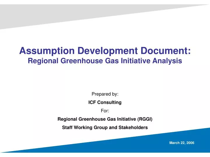
Assumption Development Document: Regional Greenhouse Gas Initiative Analysis. Prepared by: ICF Consulting For: Regional Greenhouse Gas Initiative (RGGI) Staff Working Group and Stakeholders. March 22, 2006. Outline. Project Overview Scenario Specification

E N D
Assumption Development Document:Regional Greenhouse Gas Initiative Analysis Prepared by: ICF Consulting For: Regional Greenhouse Gas Initiative (RGGI)Staff Working Group and Stakeholders March 22, 2006
Outline • Project Overview • Scenario Specification • Analytic Approach and IPM® Overview • Assumptions • Overview of Sources • Market Assumptions • Electricity Demand • Fuel Supply • Financing Assumptions • Technical Assumptions • Existing Capacity • New Fossil • Nuclear • Transmission • Pollution Control Retrofits • Renewable Capacity and Markets • Policy Assumptions • National air policy • State & regional air policy
Introduction and Goals of the Analysis • NYSERDA, on behalf of the Regional Greenhouse Gas Initiative (RGGI) Staff Working Group (SWG) has commissioned ICF Consulting to evaluate the impacts of implementing a CO2 cap on the electric power sector in the northeast and mid-Atlantic region. • The analysis that will be produced will be driven by two key issues: the Assumptions used and Scenarios examined. • Both the technical and market assumptions that serve as inputs to the modeling analysis as well as the policy scenarios evaluated have been developed by the RGGI SWG, and are the sole responsibility of the SWG. • The assumptions developed by the SWG contained in this document have been used by ICF in it’s Integrated Planning Model® (IPM®) to analyze the policies specified by the SWG. • This document provides an overview of the technical and market assumptions used for this analysis, together with documentation of the data sets that the SWG has chosen to use. • This document serves as the final assumptions document that contains all of the assumptions decided upon by the SWG for the Reference Case power sector analysis that has been conducted in the course of the RGGI process.
Purpose of this Assumptions Document • The assumptions document serves two purposes: • Introduce the structure and capabilities of the IPM® model. This document provides an overview of IPM®. It is broken out in sections discussing treatment of the elements of the electric power system within the model. Each element is defined first in terms of its role in the modeling system and then in terms of datasets that are used in the analysis. • Provide a framework to document the required assumptions. This document contains datasets from the sources for regional- and market-level assumptions that have been used in the analysis. For a study of this type, both regulatory policies and economic/technical assumptions must be defined. • Regulatory policy assumptions/specifications have been developed by the Staff Working Group. • Sources for economic and technical assumptions presented in this document include the Energy Information Administration’s Annual Energy Outlook 2005, the regional Independent System Operators (ISOs), the US EPA, and others . The Staff Working Group has reviewed and selected the sets of assumptions it feels most comfortable with. • This assumptions document presented the complete assumptions set that has been adopted by Staff Working Group assumptions.
The Challenge of Forecasting • Part of the nature of forecasting is the need to address inherently uncertain issues that have definitive impacts on the future operation of the power system. • No forecast is going to be “right” due to the fact that no one has a crystal ball regarding many of the key underlying issues, but it is extremely useful in determining directionality and cause and effect. • Policy analysis requires two things: • A Reference Case on which to base comparisons; and • Scenarios that examine the impact of changing policy, technical and market parameters. • The purpose of a Reference Case is twofold: 1) to understand system operations under existing – or expected – regulations and 2) to establish points of comparison for policy analysis. • When comparing policy/technology/market scenarios to the Reference Case, the goal should be to understand the impacts of the variables being examined. In order to understand what changes are being driven by, it is often best to change one thing at a time (isolate the variables).
Establishing a Reference Case (in RGGI Context) • “Middle-of-the-road” estimate of what the future might look like in the absence of a carbon cap-and-trade program, against which to compare the results of scenarios that contain various carbon policies. • Not a “prediction” of the future, but rather a moderate/reasonable/ plausible/ believable expectation or “best guess” for analytical purposes. • Includes existing policies, as well as those judged to be “reasonably certain or expected.” Defined to include renewable portfolio standard (RPS) programs, state regulations, and federal 3-P. • Based on current energy and environmental regulatory climate and public opinion; includes no new regulatory outcomes on either extreme that may or may not occur as a result of future debate on controversial issues.
The IPM® Modeling Framework • The Integrated Planning Model (IPM® ) was used to analyze the impacts of environmental policies on allowance markets, electric markets and compliance decisions. • IPM® is a linear programming model with a detailed representation of every boiler and generator operating in the United States. The model determines the least cost means of meeting electric energy and capacity requirements, while complying with specified air regulatory scenarios. • In addition to optimizing wholesale and environmental markets, IPM® simultaneously optimizes coal production, transportation and consumption. • IPM® contains 40 coal producing regions and has over 10 coal types defined by rank and sulfur content. • Each coal plant is assigned to one of over 40 coal demand regions characterized by location and mode of delivery including rail, barge, and truck. • Natural gas prices are derived within IPM® using a Henry Hub supply curve and regional and seasonal delivery adders.
IPM® North America NOTE: PJM-East is represented as 3 IPM® regions to separate the RGGI-affected and unaffected units in the region: PJM-East-NJ, PJM-East-Delmarva, PJM-East-PA (PECO).
Key Features of IPM® • ICF uses a national version of IPM® specifically designed for simulating the effect of environmental regulations in the electricity sector. • For this analysis, IPM® North America included a representation of at least 40 power market regions (depending on the final Northeast representation), including 10 New England regions, 5 New York regions, and 5 Canadian regions. • IPM® explicitly models transmission links between those regions. • The model includes endogenous pricing of coal supply, coal transportation and gas supply costs. • The national model determines the least cost means of complying with the specified air pollution regulations: • Multiple environmental compliance requirements are evaluated simultaneously - e.g., SO2 , NOX, CO2, Hg. • Determines optimal compliance for the system from a comprehensive range of choices including: new investment in capacity and/or pollution controls, fuel switching, repowering, retirement, and dispatch adjustments.
The IPM® Optimization Process • IPM® combines peak power demand, total energy demand, and hourly load profiles to create load duration curves for each season and region. • To meet demand, IPM® selects units to create a stack of generators dispatched by variable cost, subject to availability and other operating constraints. The last unit to be dispatched (i.e., the unit with the highest variable costs to operate) is the marginal unit and sets the energy price for that demand period. • IPM® will choose to endogenously bring to market new capacity where it is economically feasible, in order to minimize the present value costs over the lifetime of the forecast period. For example, saving 1$ in 2003 is equivalent to saving $1.60 in 2010, assuming a 7% discount rate. • All costs are prices in IPM® are represented in real 2003 dollars.
Run Years and Model Size • The high level of detail in national IPM® creates computing limitations on the overall size of the run. As a part of any modeling project, IPM® must be scoped to provide maximum resolution on the areas of interest to the client. • Various elements affect model size, but the most crucial is the number of run years. A run year is a calendar year chosen to represent a single year or a group of years that face similar electric and fuel markets and environmental policies. An IPM® run is generally limited to generating results for a maximum of 6 run years. • Because it impacts future revenue streams for generators, an updating allowance allocation mechanism requires that run years be assigned as blocks of a fixed number of calendar years, with that number corresponding to the number of years used to determine the updating allocations. • To incorporate the flexibility to run an updating allocation scenario for CO2 and to maintain the same reporting years across all scenarios and sensitivities, the run year schedule on the following slide will be adopted for the RGGI analysis. • This schedule accommodates a 3-year updating mechanism, meaning that the average generation over each 3-year block of years will be used to determine the allocation in the following 3-year block. • Due to the requirement to run the model in 3-year blocks, the start dates for some policies may need to be shifted up or back one year. The national 3-pollutant policy, for example, will be assumed to start in 2011 rather than in 2010. • Second phase cap adjustments, such as those for the 3-pollutant policy, are handled by averaging the caps over the calendar years covered by the 3-year run year block. So, that national NOX cap in the 2015 run year will be equivalent to one times the Phase I annual cap in 2014 plus 2 times the Phase II annual cap in 2015 (to represent the 2015 and 2016 caps), averaged over the 3 years.
Air Regulatory Compliance in IPM® • IPM® incorporates constraints on emissions of NOX, SO2, mercury, and CO2 into its optimization process. Constraints are specified on the basis of target-rates, cap-and-trade policies, $/ton emitted tariffs, or command-and-control policies, and applied to individual generating units or groups of units. • Units subject to constraints have a variety of compliance options: • Reduce Running Regime. In order to comply with non-command-and-control polices, a unit can limit its operational hours to more lucrative non-baseload segments. • Fuel Switch. In the case of SO2 regulations, coal and oil units can choose to burn more costly low sulfur fuels. • Retrofit. For the three current criteria pollutants (NOX, SO2, and mercury), a variety of retrofit technologies are available to reduce emissions. In the case of CO2, ICF will also model potential carbon capture-and-sequestration technologies. The cost and performance assumptions of all retrofit technologies are detailed in the Emissions Controls section below. • Retire. As with the unconstrained model, if a unit cannot cover its operating costs going forward, it is allowed to retire. • Note that units can also comply using any combination of the first three options.
Air Regulatory Treatment in IPM® • IPM® applies air emissions regulations to various classes of fossil fuel-fired generators. Regulations can vary by pollutant, structure, scope (geographic and technological), timing, and stringency. Several regulations may affect the same geographic area and, therefore, the same units. • The most common among these regulations are of the cap-and-trade type structure. Under a cap-and-trade policy, a group of units must collectively reduce their emissions to a mandated region-wide cap. For every ton of emissions up to the cap level there is a corresponding emissions allowance that can be bought or sold among affected units. Each generator complies with the program by reducing its emissions or buying allowances at the market rate, depending on the relative economics it faces. These Include the NOX SIP Call trading program and the CAAA Title IV SO2 trading program. • The other most prominent type of control policy is the Maximum Achievable Control Technology (MACT). A MACT policy requires each generator (or sometimes power plant) to control its emissions to a certain guaranteed standard rate OR install a specified control technology. The federal government is currently working on a possible MACT standard to control mercury. • IPM® can simultaneously apply a number of existing and potential future regulations restricting emissions of a variety of pollutants, including CO2.
Market, Technical and Policy Assumptions Status of Assumptions Development
IPM® New England – 10 Model Regions Based onISO-NE RTEP Definitions ME VT NH CMA/NEMA (Central / Northeast Mass) BOSTON SEMA (Southeast Mass) WMA (Western Mass) CT RI Southwest CT / Norwalk
D E B A C G H I K J IPM® Regional Breakdown of the New York A – West B – Genese C – Central D – North E – Mohawk Valley F – Capital G – Hudson Valley H – Millwood I – Dunwoodie J – NYC K – Long Island Region 1: UPSNY Region 2: CAPITAL F Region 3: DNSNY Region 5: LONG ISL. Region 4: NEW YORK CITY
PJM East* W-Cen AEP West Cinergy PJM South VIEP Kentucky IPM® Breakdown of PJM and Neighboring Regions First Energy * PJM-East is represented as 3 IPM® regions to separate the RGGI-affected and unaffected units in the region: PJM-East-NJ, PJM-East-Delmarva, PJM-East-PA (PECO)
Demand in IPM® • Demand is represented in IPM® by a combination of the following variables: • Model Demand Regions – The geographic level at which demand and supply are equilibrated to determine dispatch and prices. Each demand region acts as a power pool with a supply stack of units and a market clearing price. The proposed regional break-out for the RGGI-affected region is shown above. • Peak Demand – The maximum power load (MW) requirement for a demand region, defined by the top Demand Segment of each Season. • Energy Demand – The total energy requirement (MWh) for a demand region, defined annually. • Hourly Load Profiles – The 24-hour shape of demand level, defined for 8760 hours of a base year, for each demand region, scaled to meet peak and energy demand. Hourly load files are created from the historical load data filed by each region's utilities (FERC Form 714) for a weather normal year. • Seasons and Segments – IPM® maps annual demand, defined by hourly load profiles scaled to peak and energy demand, then breaks it into seasonal loads, defined by month. Seasonal load is further subdivided by segment. IPM® creates a dispatch stack and solves for the market clearing-price for each segment of each season in each region for each year -- 5 segments, 2 seasons, 40+ regions, and 6 “run” years will be modeled for this analysis.
Reserve Margin Assumptions • To maintain system stability and reliability, each IPM® demand region must make sure a certain amount of backup capacity is available relative to its projected peak demand. This capacity level is known as the reserve margin requirement. It is defined by a percentage of the annual peak demand. • Demand regions can meet their internal reserve margin requirements through either native supply, power imports from adjacent regions (where transmission capacity is available), or any combination of the two. • Note that the locational capacity requirements for New York City (80%) and LIPA (99%) will be imposed for this analysis. • The NYISO capacity demand curve structure will not be integrated into this analysis. • Given the focus of the RGGI analysis on mid- to long-term CO2 emissions and regulations, the demand curve is not assumed to be a critical driver in the modelled outcomes. • Because of the uncertainties facing future electric markets, including the addition of intermittent renewable capacity to the mix, growing reliance on gas, etc., the following reserve margin requirements are assumed to remain constant throughout the study period: • New York: 18% • ISO-NE: 16% • PJM: 15% • The requirements and the assumption to hold them constant were developed with the respective ISOs.
Demand and Reserve Margin Assumptions for the RGGI Analysis • The datasets chosen by the SWG for this analysis focus on the Northeast/Mid-Atlantic region that will fall under or be directly impacted by a RGGI CO2 policy, as consistent with the currently proposed geographic scope. • Because IPM® is a national model however, similar datasets must be developed for all regions in the North American system, including the Canadian regions, that are consistent with those used for the focus region. • Fuel and energy market interactions as represented in IPM® will allow behavior in the RGGI-affected regions to impact energy markets well outside the Northeast and vice-versa. Therefore, demand growth assumptions that are wholly different in the RGGI region than they are outside the RGGI region could lead to unrealistic projections. • For this reason, demand assumptions used in the RGGI regions, as taken from EIA, the relevant ISOs, or other sources, should be consistent with the growth projections to be used in the remainder of the country. • The SWG Modeling Subgroup has chosen to use ISO projections for the RGGI regions and EIA projections from AEO 2004 for the rest of the country. The following slides show the ISO projections for the RGGI-affected regions. • Because the ISOs projections do not extend past 2013 (2014 for PJM), EIA’s long-term projected growth rates, scaled to be consistent with near-term ISO growth rates, will be applied to extend the projections through the time horizon of this analysis. • The resulting scaled long-term growth rates are shown in the following slides, along with the load projections.
New York Demand Forecasts by IPM® Region Source: NYISO “2004 Load and Capacity Data” – Gold Book EIA growth rate provided as point of reference only
New England Demand Forecasts by IPM® Region Source: ISO-NE Forecast Report of Capacity, Energy, Loads and Transmission (CELT) 2004 - 2013 EIA growth rate provided as point of reference only
PJM Demand Forecasts by IPM® Region Source: PJM “2004 PJM Load Forecast Report”, Table C-1 EIA growth rate provided as point of reference only
The State Working Group has adopted a gas price trajectory phasing from a 3-year moving trend of EEA’s trajectory in the near to mid-term to a long-term EIA trajectory. To be consistent with the proposed oil price trajectory (discussed next), the EEA trend phases into an average of EIA’s natural gas projections under its AEO 2005 Reference and High Oil cases. These commodity prices are converted into delivered prices on the following slide, based on EPA seasonal and regional transportation adders. These adders are for the Reference Case(s). The adders are not assumed to change over time. Reference Case Natural Gas Price Forecast Henry Hub Gas Price (2003$/MMBtu)
Delivered Natural Gas Prices to RGGI Regions(2003$/MMBtu, Based on RGGI Year 2010 Henry Hub with EPA Base Case v.2.1.6 Transportation and Seasonality Adders)
EPA Gas Supply Curves • The ability to model natural gas price sensitivity to growing demand for gas is critical to reasonable analysis of an electric sector carbon cap. • EPA developed natural gas supply curves for use in its IPM® modeling. The curves (shown on the following page) specify annual price-volume relationships at Henry Hub wellhead and are documented on EPA’s IPM® website. • The curves were developed based on analysis using ICF’s North American Natural gas Assessment System (NANGAS) model in conjunction with electric sector gas demand generated in IPM®. • This curve structure will capture within IPM® shifts in the commodity price resulting from changes to the supply and demand of gas brought about by environmental regulation. • The EPA curves as shown, however, are likely not consistent with the price-volume relationship realized in EEA or AEO 2005. To simulate curves for this analysis based on the RGGI gas price trajectory, the slope of the EPA curves will be applied to the RGGI price projection. • The combination of the EPA curves and RGGI price projection will be made based on gas consumption results from the Reference Case for this analysis. Using this method, curves are developed that are internally consistent with the market and technical assumptions used in this analysis.
EPA Gas Supply Curves (2003$) Source: EPA Assumptions Document V.2.1.9
World Oil Price Assumptions • Oil price assumptions were developed to adequately reflect the cost of fuel switching for units that are oil- and gas-capable. • The oil price projection for the RGGI analysis is based on EIA AEO 2005 projections and adjusted as follows: • In the near-term, EIA’s AEO 2005 world oil price forecast is scaled by the relative gas prices (AEO as compared to the RGGI trajectory) to arrive at a modified EIA trajectory. • In the long-term (2015 and later), the trajectory is equal to the average of EIA’s Reference Case and High Oil Case projections. • EIA’s world oil price is the annual average U.S. refiner’s acquisition cost of imported crude oil. • The outcome of this adjustment is shown on the following slide and compared to the proposed gas price trajectory.
World Oil Price Assumptions continued World Oil Price: Proposed Henry Hub Gas Price: Proposed
Delivered Oil Price Assumptions • Delivered product prices are derived from the assumed world oil price shown on the previous slide and an analysis of historical price relationships and delivered prices. • The 0.3%S price trajectory was derived based on a regression of product prices to world crude prices over 6 years (1998 through 2003). • The price differential between 0.3%S and 1.0%S is assumed to remain constant over time and is equal to the 6-year average historical differential between the two products. • Delivered prices for both products are based on historical data for select cities. • The following slide compares delivered oil and gas prices in 2010 for the RGGI region. The two following slides show time series projections for two select regions.
Coal Supply and Demand Analytic ApproachOverview • Coal supply curves are used in IPM® to capture price and production responses from fuel switching for environmental compliance. • ICF has developed supply curves (described later in this section) for use in its analyses. To be consistent with the long-term gas and oil prices in this analysis, the SWG chose to calibrate these curves to EIA’s AEO 2004 coal price and production results. • Like gas and oil prices, near-term (2005 and 2006) coal prices have also been calibrated to current future markets to reflect present market conditions not captured in EIA’s projections. • Current commodity price premiums and transportation bottlenecks are assumed to ease over time as export markets for U.S. coal come into balance and domestic production increases. • The tables at right show the price projections for key coals that the supply curves have been calibrated to. The actual prices realized in the modeling will depend on the assumed environmental regulations and other market conditions. • Delivered prices of these coals to New York, New England and Pennsylvania are shown on the following slide, along with the emissions and energy characteristics of each coal. • Because reliable spot pricing and characteristics are not readily available, international coals will not be represented in this process.
Coal Supply and Demand Analytic ApproachIPM® Coal Market Structure • Coal resources for each of 40 coal supply basins are disaggregated into the following categories: • Rank • Sulfur content • Existing and new • Surface: Overburden Ratio, Size, Mining Method • Underground: Depth, Seam Thickness, Mining Method • Mercury contents are assigned to coals by rank and production region based on EPA’s 1999 ICR shipment data. • Coal supply curves for each of the 40 supply basins are created by applying disaggregated coal resources assigned to one of 16 prototype coal costing models. • The coal supply curves are then used as inputs to IPM®. • Coal plants in IPM® are assigned to one of 41 different coal demand regions that are defined by location and mode of delivery. • A coal transportation matrix links supply and demand regions in IPM®, which determines the least cost means to meet power demand for coal as part of an integrated optimal solution for power, fuel, and emission markets. IPM® Coal Supply Regions
Discount Rate • IPM® is a linear programming model that optimizes system performance in a least cost manner to meet any number of market and policy requirements (constraints) defined in the analysis. • All costs in the model are represented in real 2003$, and are then discounted back on a present value basis to determine the least cost way to meet the market and policy requirements defined. The discount rate then becomes important in evaluating the tradeoffs of making investments and incurring costs in the near-term vs. incurring expenses over the longer-term. • For this analysis, the SWG chose to use a 6.86% (real) discount rate on a system-wide basis to evaluate revenues and costs and to make investment decisions.
Financial Assumptions • Capital investments in IPM® are annualized using a capital charge rate that takes into account the ratio of debt and equity and their respective rates, taxes, depreciation schedule, book life and debt life. Capital charge rates are assigned to each technology type as shown on the next slide. • The assumptions shown on the following page are intended to reflect financial conditions characteristic of merchant investments, or those investments likely to be the marginal decisions that IPM® relies on to forecast energy and capacity prices. • New gas- and coal-fired capacity options are assumed to face similar debt rate and return-on-equity requirements. Investments in new nuclear capacity are assumed to require higher rates to account for a higher risk profile. Pollution control options, because they will be installed on existing units with available historical generation and cost profiles, are assumed to be financed at lower rates.
Financial Assumptions For Potential Builds and Retrofits * Also applies to repowering options from coal and oil/gas steam units to new combined cycle units. NOTE: Income tax and other tax/insurance rates updated as of July 2003.