Download
1 / 103
1.05k likes | 1.49k Views
Strategy for Complete Regression Analysis. Additional issues in regression analysis Assumption of independence of errors Influential cases Multicollinearity Adjusted R² Strategy for Solving problems Sample problems Complete regression analysis. Assumption of independence of errors - 1.

E N D
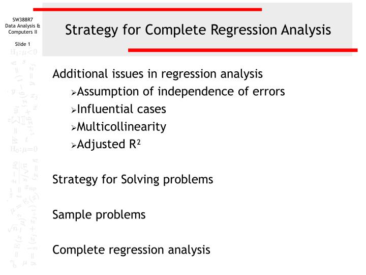
Strategy for Complete Regression Analysis Additional issues in regression analysis Assumption of independence of errors Influential cases Multicollinearity Adjusted R² Strategy for Solving problems Sample problems Complete regression analysis
Assumption of independence of errors - 1 • Multiple regression assumes that the errors are independent and there is no serial correlation. Errors are the residuals or differences between the actual score for a case and the score estimated using the regression equation. No serial correlation implies that the size of the residual for one case has no impact on the size of the residual for the next case. • The Durbin-Watson statistic is used to test for the presence of serial correlation among the residuals. The value of the Durbin-Watson statistic ranges from 0 to 4. As a general rule of thumb, the residuals are not correlated if the Durbin-Watson statistic is approximately 2, and an acceptable range is 1.50 - 2.50.
Assumption of independence of errors - 2 • Serial correlation is more of a concern in analyses that involve time series. • If it does occur in relationship analyses, its presence can be usually be understood by changing the sequence of cases and running the analysis again. • If the problem with serial correlation disappears, it may be ignored. • If the problem with serial correlation remains, it can usually be handled by using the difference between successive data points as the dependent variable.
Multicollinearity - 1 • Multicollinearity is a problem in regression analysis that occurs when two independent variables are highly correlated, e.g. r = 0.90, or higher. • The relationship between the independent variables and the dependent variables is distorted by the very strong relationship between the independent variables, leading to the likelihood that our interpretation of relationships will be incorrect. • In the worst case, if the variables are perfectly correlated, the regression cannot be computed. • SPSS guards against the failure to compute a regression solution by arbitrarily omitting the collinear variable from the analysis.
Multicollinearity - 2 • Multicollinearity is detected by examining the tolerance for each independent variable. Tolerance is the amount of variability in one independent variable that is no explained by the other independent variables. • Tolerance values less than 0.10 indicate collinearity. • If we discover collinearity in the regression output, we should reject the interpretation of the relationships as false until the issue is resolved. • Multicollinearity can be resolved by combining the highly correlated variables through principal component analysis, or omitting a variable from the analysis.
Adjusted R² • The coefficient of determination, R² which measures the strength of a relationship, can usually be increased simply by adding more variables. In fact, if the number of variables equals the number of cases, it is often possible to produce a perfect R² of 1.00. • Adjusted R² is a measure which attempts to reduce the inflation in R² by taking into account the number of independent variables and the number of cases. • If there is a large discrepancy between R² and Adjusted R², extraneous variables should be removed from the analysis and R² recomputed.
Influential cases • The degree to which outliers affect the regression solution depends upon where the outlier is located relative to the other cases in the analysis. Outliers whose location have a large effect on the regression solution are called influential cases. • Whether or not a case is influential is measured by Cook’s distance. • Cook’s distance is an index measure; it is compared to a critical value based on the formula: 4 / (n – k – 1) where n is the number of cases and k is the number of independent variables. • If a case has a Cook’s distance greater than the critical value, it should be examined for exclusion.
Overall strategy for solving problems • Run a baseline regression using the method for including variables implied by the problem statement to find the initial strength of the relationship, baseline R². • Test for useful transformations to improve normality, linearity, and homoscedasticity. • Substitute transformed variables and check for outliers and influential cases. • If R² from regression model using transformed variables and omitting outliers is at least 2% better than baseline R², select it for interpretation; otherwise select baseline model. • Validate and interpret the selected regression model.
Problem 1 In the dataset GSS2000.sav, is the following statement true, false, or an incorrect application of a statistic? Assume that there is no problem with missing data. Use a level of significance of 0.05 for the regression analysis. Use a level of significance of 0.01 for evaluating assumptions. Use 0.0160 as the criteria for identifying influential cases. Validate the results of your regression analysis by splitting the sample in two, using 788035 as the random number seed. The variables "age" [age], "sex" [sex], and "respondent's socioeconomic index" [sei] have a strong relationship to the variable "how many in family earned money" [earnrs]. Survey respondents who were older had fewer family members earning money. The variables sex and respondent's socioeconomic index did not have a relationship to how many in family earned money. 1. True 2. True with caution 3. False 4. Inappropriate application of a statistic
Dissecting problem 1 - 1 When we test for influential cases using Cook’s distance, we need to compute a critical value for comparison using the formula: 4 / (n – k – 1) where n is the number of cases and k is the number of independent variables. The correct value (0.0160) is provided in the problem. The problem may give us different levels of significance for the analysis. In this problem, we are told to use 0.05 as alpha for the regression, but 0.01 for testing assumptions. In the dataset GSS2000.sav, is the following statement true, false, or an incorrect application of a statistic? Assume that there is no problem with missing data. Use a level of significance of 0.05 for the regression analysis. Use a level of significance of 0.01 for evaluating assumptions. Use 0.0160 as the criteria for identifying influential cases. Validate the results of your regression analysis by splitting the sample in two, using 788035 as the random number seed. The variables "age" [age], "sex" [sex], and "respondent's socioeconomic index" [sei] have a strong relationship to the variable "how many in family earned money" [earnrs]. After evaluating assumptions, outliers, and influential cases, we will decide whether we should use the model with transformations and excluding outliers, or the model with the original form of the variables and all cases. The random number seed (788035) for the split sample validation is provided.
Dissecting problem 1 - 2 The variables listed first in the problem statement are the independent variables (IVs): "age" [age], "sex" [sex], and "respondent's socioeconomic index" [sei]. When a problem states that there is a relationship between some independent variables and a dependent variable, we do standard multiple regression. In the dataset GSS2000.sav, is the following statement true, false, or an incorrect application of a statistic? Assume that there is no problem with missing data. Use a level of significance of 0.05 for the regression analysis. Use a level of significance of 0.01 for evaluating assumptions. Use 0.0160 as the criteria for identifying influential cases. Validate the results of your regression analysis by splitting the sample in two, using 788035 as the random number seed. The variables "age" [age], "sex" [sex], and "respondent's socioeconomic index" [sei] have a strong relationship to the variable "how many in family earned money" [earnrs]. Survey respondents who were older had fewer family members earning money. The variables sex and respondent's socioeconomic index did not have a relationship to how many in family earned money. 1. True 2. True with caution 3. False 4. Inappropriate application of a statistic The variable that is the target of the relationship is the dependent variable (DV): "how many in family earned money“ [earnrs].
Dissecting problem 1 - 3 In order for a problem to be true, we will have to find that there is a statistically significant relationship between the set of IVs and the DV, and the strength of the relationship stated in the problem must be correct. In the dataset GSS2000.sav, is the following statement true, false, or an incorrect application of a statistic? Assume that there is no problem with missing data. Use a level of significance of 0.05 for the regression analysis. Use a level of significance of 0.01 for evaluating assumptions. Use 0.0160 as the criteria for identifying influential cases. Validate the results of your regression analysis by splitting the sample in two, using 788035 as the random number seed. The variables "age" [age], "sex" [sex], and "respondent's socioeconomic index" [sei] have a strong relationship to the variable "how many in family earned money" [earnrs]. Survey respondents who were older had fewer family members earning money. The variables sex and respondent's socioeconomic index did not have a relationship to how many in family earned money. 1. True 2. True with caution 3. False 4. Inappropriate application of a statistic In addition, the relationship or lack of relationship between the individual IV's and the DV must be identified correctly, and must be characterized correctly.
LEVEL OF MEASUREMENT Multiple regression requires that the dependent variable be metric and the independent variables be metric or dichotomous. In the dataset GSS2000.sav, is the following statement true, false, or an incorrect application of a statistic? Assume that there is no problem with missing data. Use a level of significance of 0.05 for the regression analysis. Use a level of significance of 0.01 for evaluating assumptions. Use 0.0160 as the criteria for identifying influential cases. Validate the results of your regression analysis by splitting the sample in two, using 788035 as the random number seed. The variables "age" [age], "sex" [sex], and "respondent's socioeconomic index" [sei] have a strong relationship to the variable "how many in family earned money" [earnrs]. Survey respondents who were older had fewer family members earning money. The variables sex and respondent's socioeconomic index did not have a relationship to how many in family earned money. 1. True 2. True with caution 3. False 4. Inappropriate application of a statistic "How many in family earned money" [earnrs] is an interval level variable, which satisfies the level of measurement requirement. "Age" [age] and "respondent's socioeconomic index" [sei] are interval level variables, which satisfies the level of measurement requirements for multiple regression analysis. "Sex" [sex] is a dichotomous or dummy-coded nominal variable which may be included in multiple regression analysis.
The baseline regression We begin out analysis by runring a standard multiple regression analysis with earnrs as the dependent variable and age, sex, and sei as the independent variables. Select Enter as the Method for including variables to produce a standard multiple regression. Click on the Statistics… button to select statistics we will need for the analysis.
The baseline regression Retain the default checkboxes for Estimates and Model fit to obtain the baseline R², which will be used to determine whether we should use the model with transformations and excluding outliers, or the model with the original form of the variables and all cases. Mark the Descriptives checkbox to get the number of cases available for the analysis. Mark the checkbox for the Durbin-Watson statistic, which will be used to test the assumption of independence of errors.
Initial sample size The initial sample size before excluding outliers and influential cases is 254. With 3 independent variables, the ratio of cases to variables is 84.7 to 1, satisfying both the minimum and preferred sample size for multiple regression. If the sample size did not initially satisfy the minimum requirement, regression analysis is not appropriate.
R² before transformations or removing outliers The R² of 0.187 is the benchmark that we will use to evaluate the utility of transformations and the elimination of outliers/influential cases. Prior to any transformations of variables to satisfy the assumptions of multiple regression or removal of outliers, the proportion of variance in the dependent variable explained by the independent variables (R²) was 18.7%. The relationship is statistically significant, though we would not stop if it were not significant because the lack of significance may be a consequence of violation of assumptions or the inclusion of outliers and influential cases.
Assumption of independence of errors:the Durbin-Watson statistic The Durbin-Watson statistic is used to test for the presence of serial correlation among the residuals, i.e., the assumption of independence of errors, which requires that the residuals or errors in prediction do not follow a pattern from case to case. The value of the Durbin-Watson statistic ranges from 0 to 4. As a general rule of thumb, the residuals are not correlated if the Durbin-Watson statistic is approximately 2, and an acceptable range is 1.50 - 2.50. The Durbin-Watson statistic for this problem is 1.849 which falls within the acceptable range. If the Durbin-Watson statistic was not in the acceptable range, we would add a caution to the findings for a violation of regression assumptions.
Normality of dependent variable:how many in family earned money After evaluating the dependent variable, we examine the normality of each metric variable and linearity of its relationship with the dependent variable. To test the normality of number of earners in family, run the script: NormalityAssumptionAndTransformations.SBS First, move the independent variable EARNRS to the list box of variables to test. Second, click on the OK button to produce the output.
Normality of dependent variable:how many in family earned money The dependent variable "how many in family earned money" [earnrs] does not satisfy the criteria for a normal distribution. The skewness (0.742) fell between -1.0 and +1.0, but the kurtosis (1.324) fell outside the range from -1.0 to +1.0.
Normality of dependent variable:how many in family earned money The logarithmic transformation improves the normality of "how many in family earned money" [earnrs]. In evaluating normality, the skewness (-0.483) and kurtosis (-0.309) were both within the range of acceptable values from -1.0 to +1.0. The square root transformation also has values of skewness and kurtosis in the acceptable range. However, by our order of preference for which transformation to use, the logarithm is preferred to the square root or inverse.
Transformation for how many in family earned money • The logarithmic transformation improves the normality of "how many in family earned money" [earnrs]. • We will substitute the logarithmic transformation of how many in family earned money as the dependent variable in the regression analysis.
Adding a transformed variable Before testing the assumptions for the independent variables, we need to add the transformation of the dependent variable to the data set. First, move the variable that we want to transform to the list box of variables to test. Second, mark the checkbox for the transformation we want to add to the data set, and clear the other checkboxes. Third, clear the checkbox for Delete transformed variables from the data. This will save the transformed variable. Fourth, click on the OK button to produce the output.
The transformed variable in the data editor If we scroll to the extreme right in the data editor, we see that the transformed variable has been added to the data set. Whenever we add transformed variables to the data set, we should be sure to delete them before starting another analysis.
Normality/linearity of independent variable: age After evaluating the dependent variable, we examine the normality of each metric variable and linearity of its relationship with the dependent variable. To test the normality of age, run the script: NormalityAssumptionAndTransformations.SBS First, move the independent variable AGE to the list box of variables to test. Second, click on the OK button to produce the output.
Normality/linearity of independent variable: age In evaluating normality, the skewness (0.595) and kurtosis (-0.351) were both within the range of acceptable values from -1.0 to +1.0.
Normality/linearity of independent variable: age First, move the transformed dependent variable LOGEARN to the text box for the dependent variable. To evaluate the linearity of age and the log transformation of number of earners in the family, run the script for the assumption of linearity: LinearityAssumptionAndTransformations.SBS Second, move the independent variable, AGE, to the list box for independent variables. Third, click on the OK button to produce the output.
Normality/linearity of independent variable: age The evidence of linearity in the relationship between the independent variable "age" [age] and the dependent variable "log transformation of how many in family earned money" [logearn] was the statistical significance of the correlation coefficient (r = -0.493). The probability for the correlation coefficient was <0.001, less than or equal to the level of significance of 0.01. We reject the null hypothesis that r = 0 and conclude that there is a linear relationship between the variables. The independent variable "age" [age] satisfies the criteria for both the assumption of normality and the assumption of linearity with the dependent variable "log transformation of how many in family earned money" [logearn].
Normality/linearity of independent variable: respondent's socioeconomic index First, move the independent variable SEI to the list box of variables to test. To test the normality of respondent's socioeconomic index, run the script: NormalityAssumptionAndTransformations.SBS Second, click on the OK button to produce the output.
Normality/linearity of independent variable: respondent's socioeconomic index The independent variable "respondent's socioeconomic index" [sei] satisfies the criteria for the assumption of normality, but does not satisfy the assumption of linearity with the dependent variable "log transformation of how many in family earned money" [logearn]. In evaluating normality, the skewness (0.585) and kurtosis (-0.862) were both within the range of acceptable values from -1.0 to +1.0.
Normality/linearity of independent variable: respondent's socioeconomic index First, move the transformed dependent variable LOGEARN to the text box for the dependent variable. To evaluate the linearity of the relationship between respondent's socioeconomic index and the log transformation of how many in family earned money, run the script for the assumption of linearity: LinearityAssumptionAndTransformations.SBS Second, move the independent variable, SEI, to the list box for independent variables. Third, click on the OK button to produce the output.
Normality/linearity of independent variable: respondent's socioeconomic index The probability for the correlation coefficient was 0.385, greater than the level of significance of 0.01. We cannot reject the null hypothesis that r = 0, and cannot conclude that there is a linear relationship between the variables. Since none of the transformations to improve linearity were successful, it is an indication that the problem may be a weak relationship, rather than a curvilinear relationship correctable by using a transformation. A weak relationship is not a violation of the assumption of linearity, and does not require a caution.
Homoscedasticity of independent variable: Sex First, move the transformed dependent variable LOGEARN to the text box for the dependent variable. To evaluate the homoscedasticity of the relationship between sex and the log transformation of how many in family earned money, run the script for the assumption of homogeneity of variance: HomoscedasticityAssumptionAnd Transformations.SBS Second, move the independent variable, SEX, to the list box for independent variables. Third, click on the OK button to produce the output.
Homoscedasticity of independent variable: Sex Based on the Levene Test, the variance in "log transformation of how many in family earned money" [logearn] is homogeneous for the categories of "sex" [sex]. The probability associated with the Levene Statistic (0.767) is greater than the level of significance, so we fail to reject the null hypothesis and conclude that the homoscedasticity assumption is satisfied.
The regression to identify outliers and influential cases We use the regression procedure to identify univariate outliers, multivariate outliers, and influential cases. We start with the same dialog we used for the baseline analysis and substitute the transformed variables which we think will improve the analysis. To run the regression again, select the Regression | Linear command from the Analyze menu.
The regression to identify outliers and influential cases First, we substitute the logarithmic transformation of earnrs, logearn, into the list of independent variables. Second, we keep the method of entry to Enter so that all variables will be included in the detection of outliers. NOTE: we should always use Enter when testing for outliers and influential cases to make sure all variables are included in the determination. Third, we want to save the calculated values of the outlier statistics to the data set. Click on the Save… button to specify what we want to save.
Saving the measures of outliers/influential cases First, mark the checkbox for Studentized residuals in the Residuals panel. Studentized residuals are z-scores computed for a case based on the data for all other cases in the data set. Fourth, click on the OK button to complete the specifications. Second, mark the checkbox for Mahalanobis in the Distances panel. This will compute Mahalanobis distances for the set of independent variables. Third, mark the checkbox for Cook’s in the Distances panel. This will compute Cook’s distances to identify influential cases.
The variables for identifying outliers/influential cases The variable for identifying univariate outliers for the dependent variable are in a column which SPSS has named sre_1. These are the studentized residuals for the log transformed variables. The variable for identifying multivariate outliers for the independent variables are in a column which SPSS has named mah_1. The variable containing Cook’s distances for identifying influential cases has been named coo_1 by SPSS.
Computing the probability for Mahalanobis D² To compute the probability of D², we will use an SPSS function in a Compute command. First, select the Compute… command from the Transform menu.
Formula for probability for Mahalanobis D² First, in the target variable text box, type the name "p_mah_1" as an acronym for the probability of the mah_1, the Mahalanobis D² score. Second, to complete the specifications for the CDF.CHISQ function, type the name of the variable containing the D² scores, mah_1, followed by a comma, followed by the number of variables used in the calculations, 3. Since the CDF function (cumulative density function) computes the cumulative probability from the left end of the distribution up through a given value, we subtract it from 1 to obtain the probability in the upper tail of the distribution. Third, click on the OK button to signal completion of the computer variable dialog.
Univariate outliers A score on the dependent variable is considered unusual if its studentized residual is bigger than ±3.0.
Multivariate outliers The combination of scores for the independent variables is an outlier if the probability of the Mahalanobis D² distance score is less than or equal to 0.001.
Influential cases In addition, a case may have a large influence on the regression analysis, resulting in an analysis that is less representative of the population represented by the sample. The criteria for identifying influential case is a Cook's distance score with a value of 0.0160 or greater. The criteria for Cook’s distance is: 4 / (n – k – 1) = 4 / (254 – 3 – 1) = 0.0160
Omitting the outliers and influential cases To omit the outliers and influential cases from the analysis, we select in the cases that are not outliers and are not influential cases. First, select the Select Cases… command from the Transform menu.
Specifying the condition to omit outliers First, mark the If condition is satisfied option button to indicate that we will enter a specific condition for including cases. Second, click on the If… button to specify the criteria for inclusion in the analysis.
The formula for omitting outliers To eliminate the outliers and influential cases, we request the cases that are not outliers or influential cases. The formula specifies that we should include cases if the studentized residual (regardless of sign) is less than 3, the probability for Mahalanobis D² is higher than the level of significance of 0.001, and the Cook’s distance value is less than the critical value of 0.0160. After typing in the formula, click on the Continue button to close the dialog box,
Completing the request for the selection To complete the request, we click on the OK button.
An omitted outlier and influential case SPSS identifies the excluded cases by drawing a slash mark through the case number. This omitted case has a large studentized residual, greater than 3.0, as well as a Cook’s distance value that is greater than the critical value, 0.0160.
The outliers and influential cases Case 20000159 is an influential case (Cook's distance=0.0320) as well as an outlier on the dependent variable (studentized residual=3.13). Case 20000915 is an influential case (Cook's distance=0.0239). Case 20001016 is an influential case (Cook's distance=0.0598) as well as an outlier on the dependent variable (studentized residual=-3.12). Case 20001761 is an influential case (Cook's distance=0.0167). Case 20002587 is an influential case (Cook's distance=0.0264). Case 20002597 is an influential case (Cook's distance=0.0293). There are 6 cases that have a Cook's distance score that is large enough to be considered influential cases.
Running the regression omitting outliers We run the regression again, without the outliers which we selected out with the Select If command. Select the Regression | Linear command from the Analyze menu.