Download
1 / 27
280 likes | 388 Views
Forecasting (prediction) limits. Example Linear deterministic trend estimated by least-squares. Note! The average of the numbers 1, 2, … , t is. Hence, calculated prediction limits for Y t+l become where c is a quantile of a proper sampling distribution emerging from the use of

E N D
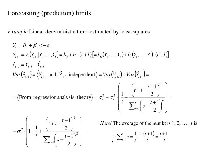
Forecasting (prediction) limits Example Linear deterministic trend estimated by least-squares Note! The average of the numbers 1, 2, … , t is
Hence, calculated prediction limits for Yt+l become where c is a quantile of a proper sampling distribution emerging from the use of and the requested coverage of the limits. For t large it suffices to use the standard normal distribution and a good approximation is also obtained even if the term is omitted under the square root
ARIMA-models Using R ts=arima(x,…) for fitting models plot.Arima(ts,…) for plotting fitted models with 95% prediction limits See documentation for plot.Arima . However, the generic command plot can be used. forecast.Arima Install and load package “forecast”. Gives more flexibility with respect to prediction limits.
Seasonal ARIMA models Example “beersales” data A clear seasonal pattern and also a trend, possibly a quadratic trend
Residuals from detrended data beerq<-lm(beersales~time(beersales)+I(time(beersales)^2)) plot(y=rstudent(beerq),x=as.vector(time(beersales)),type="b", pch=as.vector(season(beersales)),xlab="Time") Seasonal pattern, but possibly no long-term trend left
SAC and SPAC of the residuals: SAC Spikes at or close to seasonal lags (or half-seasonal lags) SPAC
Modelling the autocorrelation at seasonal lags Pure seasonal variation:
Non-seasonal and seasonal variation: AR(p, P)s or ARMA(p,0)(P,0)s However, we cannot discard that the non-seasonal and seasonal variation “interact” Better to use multiplicative Seasonal AR Models Example:
Multiplicative MA(q, Q)s or ARMA(0,q)(0,Q)s Mixed models: Many terms! Condensed expression:
Non-stationary Seasonal ARIMA models Non-stationary at non-seasonal level: Model dth order regular differences: Non-stationary at seasonal level: Seasonal non-stationarity is harder to detect from a plotted times-series. The seasonal variation is not stable. Model Dth order seasonal differences: Example First-order monthly differences: can follow a stable seasonal pattern
The general Seasonal ARIMA model It does not matter whether regular or seasonal differences are taken first
Model specification, fitting and diagnostic checking Example “beersales” data Clearly non-stationary at non-seasonal level, i.e. there is a long-term trend
Investigate SAC and SPAC of original data Many substantial spikes both at non-seasonal and at seasonal level- Calls for differentiation at both levels.
Try first-order seasonal differences first. Here: monthly data beer_sdiff1 <- diff(beersales,lag=12) Look at SAC and SPAC again Better, but now we need to try regular differences
Take first order differences in seasonally differenced data beer_sdiff1rdiff1 <- diff(beer_sdiff1,lag=1) Look at SAC and SPAC again SAC starts to look “good”, but SPAC not
Take second order differences in seasonally differenced data Since we suspected a non-linear long-term trend beer_sdiff1rdiff2 <- diff(diff(beer_sdiff1,lag=1),lag=1) Non-seasonal part Seasonal part Could be an ARMA(2,0)(0,1)12 or an ARMA(1,1) (0,1)12
These models for original data becomes ARIMA(2,2,0) (0,1,1)12 and ARIMA(1,2,1) (0,1,1)12 model1 <-arima(beersales,order=c(2,2,0), seasonal=list(order=c(0,1,1),period=12)) Series: beersales ARIMA(2,2,0)(0,1,1)[12] Coefficients: ar1 ar2 sma1 -1.0257 -0.6200 -0.7092 s.e. 0.0596 0.0599 0.0755 sigma^2 estimated as 0.6095: log likelihood=-216.34 AIC=438.69 AICc=438.92 BIC=451.42
Diagnostic checking can be used in a condensed way by function tsdiag. The Ljung-Box test can specifically be obtained from function Box.test tsdiag(model1) standardized residuals SPAC(standardized residuals) P-values of Ljung-Box test with K = 24
Box.test(residuals(model1), lag = 12, type = "Ljung-Box", fitdf = 3) Box-Ljung test data: residuals(model1) X-squared = 30.1752, df = 9, p-value = 0.0004096 K (how many lags included) p + q + P + Q (how many degrees of freedom withdrawn from K) For seasonal data with season length s the L-B test is usually calculated for K = s, 2s, 3s and 4s
Box.test(residuals(model1), lag = 24, type = "Ljung-Box", fitdf = 3) Box-Ljung test data: residuals(model1) X-squared = 57.9673, df = 21, p-value = 2.581e-05 Box.test(residuals(model1), lag = 36, type = "Ljung-Box", fitdf = 3) Box-Ljung test data: residuals(model1) X-squared = 76.7444, df = 33, p-value = 2.431e-05 Box.test(residuals(model1), lag = 48, type = "Ljung-Box", fitdf = 3) Box-Ljung test data: residuals(model1) X-squared = 92.9916, df = 45, p-value = 3.436e-05
Hence, the residuals from the first model are not satisfactory model2 <-arima(beersales,order=c(1,2,1), seasonal=list(order=c(0,1,1),period=12)) print(model2) Series: beersales ARIMA(1,2,1)(0,1,1)[12] Coefficients: ar1 ma1 sma1 -0.4470 -0.9998 -0.6352 s.e. 0.0678 0.0176 0.0930 sigma^2 estimated as 0.4575: log likelihood=-192.86 AIC=391.72 AICc=391.96 BIC=404.45 Better fit ! But is it good?
tsdiag(model2) Not good! We should maybe try second-order seasonal differentiation too.
Time series regression models The classical set-up uses deterministic trend functions and seasonal indices The classical set-up can be extended by allowing for autocorrelated error terms (instead of white noise). Usually it is sufficient with and AR(1) or AR(2). However, the trend and seasonal terms are still assumed deterministic.
Dynamic time series regression models To extend the classical set-up with explanatory variables comprising other time series we need another way of modelling. Note that a stationary ARMA-model can also be written
The general dynamic regression model for a response time series Ytwith one covariate time series Xtcan be written Special case 1: Xtrelates to some event that has occurred at a certain time points (e.g. 9/11) It can the either be a step function or a pulse function
Step functions would imply a permanent change in the level of Yt. Such a change can further be constant or gradually increasing (depending on (B) and (B) ). It can also be delayed (depending on b ) • Pulse functions would imply a temporary change in the level of Yt . Such a change may be just at the specific time point gradually decreasing (depending on (B) and (B) ). • Strep and pulse functions are used to model the effects of a particular event, as so-called intervention. • Intervention models • For Xt being a “regular” times series (i.e. varying with time) the models are called transfer function models