Download
1 / 90
920 likes | 1.14k Views
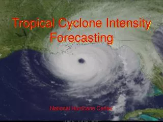
NATIONAL CENTERS FOR ENVIRONMENTAL PREDICTION. Tropical Cyclone Track Forecasting. Jamie Rhome WMO Workshop National Hurricane Center. NATIONAL CENTERS FOR ENVIRONMENTAL PREDICTION WHERE AMERICA’S CLIMATE AND WEATHER SERVICES BEGIN. OUTLINE: TRACK FORECASTING. Factors affecting TC motion

E N D
NATIONAL CENTERS FOR ENVIRONMENTAL PREDICTION Tropical Cyclone Track Forecasting Jamie Rhome WMO Workshop National Hurricane Center NATIONAL CENTERS FOR ENVIRONMENTAL PREDICTION WHERE AMERICA’S CLIMATE AND WEATHER SERVICES BEGIN
OUTLINE: TRACK FORECASTING • Factors affecting TC motion • Guidance Models • Climatology and Statistical models • Beta and Advection Models • Dynamical Models • Ensembles and Consensus • NHC Forecasting Guidelines • Using Initial Motion • Continuity • Bringing it All Together: Interpreting Track Models • Exercise
Factors Affecting TC Motion: • Large-scale • Vortex Moves with “Steering Flow” main contributor to TC motion • Cyclone-scale • Vortex induces beta-gyres and other asymmetries that affect motion • Convective distribution • Vertical Structure • Other • Binary interaction (Fujiwhara effect) • Landmass interaction • Internal dynamics (trochoidal motion)
The Large-scale Steering Flow is the Main Contributor to TC Motion H L L
The Beta Effect • The circulation of a TC, combined with the North-South variation of the Coriolis parameter, induces asymmetries known as Beta Gyres. INDUCED STEERING 1-2 m/s NW HIGHER VALUES OF EARTH’S VORTICITY H βv>0 • Beta Gyres produce a net steering current across the TC, generally toward the NW at a few knots. This motion is knows as the Beta Drift. βv<0 L N LOWER VALUES OF EARTH’S VORTICITY
Binary Interaction (Fujiwhara Effect) Relative rotation diagram of 12-h positions relative to the midpoints between Bopha (in solid typhoon symbol) and Saomai (in solid dot) based on a direct binary interaction interpretation (Wu et. al, 2003) • Fujiwhara effect—Occurs when two tropical cyclones become close enough (< 1450 km) to rotate cyclonically about each other as a result of their circulations' mutual advection. • Named after Dr. Sakuhei Fujiwhara who initially described it in a 1921 paper about the motion of vortices in water • Most often occurs in the northwestern and eastern North Pacific basin…less often in the Atlantic. • Presents a unique forecast challenge since the complex interplay results in different scenarios which determine the final result of the interaction • Some of the factors affecting the outcome of binary interaction include: comparable strength of the two cyclones, comparable size of the two cyclones, distance apart, background flow
Trochoidal Motion (Wobble) • Related to inner-core structure, convective asymmetries, and dynamic instability • Unable to forecast • Simply observe • Beware of the “wobble” • Wait for a sustained (several hours) change in motion
Hierarchy of TC Track Guidance Models: • Statistical • Forecasts based on established relationships between storm-specific information (i.e., location and time of year) and the behavior of previous storms • CLIPER • Statistical-Dynamical • Statistical models that use information from dynamical model output • NHC91 still maintains skill in the eastern Pacific • Simplified Dynamical • LBAR simple two-dimensional dynamical track prediction model that solves the shallow-water equations initialized with vertically averaged (850-200 hPa) winds and heights from the GFS global model • BAMD, BAMM, BAMS -> Forecasts based on simplified dynamic representation of interaction with vortex and prevailing flow (trajectory) • Dynamical Models • Solve the physical equations of motion that govern the atmosphere • GFDL, GFDN, GFS, NOGAPS, UKMET, ECMWF, NAM, (HWRF)
CLIPER (CLImatology and PERsistence) Model Statistical track model developed in 1972, extended to 120 h in 1998 Required Input: Current/12 h old speed/direction of motion Current latitude/longitude Julian Day, Storm maximum wind Average 24, 48, 72, 96 and 120 h errors: 100, 216, 318, 419, and 510 nautical miles respectively Used as a benchmark for other models and subjective forecasts; forecasts with errors greater than CLIPER are considered to have no skill.
Beta and Advection Model (BAM) • Method: Steering (trajectories) given by layer-averaged winds from a global model (horizontally smoothed to T25 resolution), plus a correction term to simulate the so-called “Beta Effect” • Three different layer averages: • Shallow (850-700 MB) - BAMS • Medium (850-400 MB) - BAMM • Deep (850-200 MB) - BAMD
DEEP MEDIUM SHALLOW L L L TROPICAL STORM / CAT. 1-2 HURRICANE MAJOR HURRICANE WHICH BAM TO USE? 200 mb Typical cruising altitude of commercial airplane 400 mb 700 mb Surface TROPICAL DEPRESSION 5,000 ft/850 mb
LBAR (Limited-area BARotropic) • Barotropic dynamics, i.e. 2-d motions – no temperature gradients or vertical shear • Lack of baroclinic forcing means the model has little or no skill beyond 1-2 days • Shallow water equations on Mercator projection solved using sine transforms • Initialized with 850-200 mb layer average winds/heights from NCEP global model (GFS) • Sum of idealized vortex and current motion vector added to large-scale analysis • Boundary conditions from global model
Primary Dynamical Models used at NHC • U.S. NWS Global Forecast System (GFS) < relocates the first-guess TC vortex • United Kingdom Met. Office (UKMET) < bogus (syn. data) • U.S. Navy Operational Global Atmospheric Prediction System (NOGAPS) < bogus (syn. data) • U.S. NWS Geophysical Fluid Dynamics Laboratory (GFDL) model <bogus (spinup vortex) • GFDN- Navy version of GFDL <bogus (spinup vortex) • European Center for Medium-range Weather Forecasting (ECMWF) model (no bogus)
Bogussing • Since the globally analyzed vortex does not typically represent the structure of a true TC, “Bogussing” is often employed. • Bogussing involves an analysis of synthetic data to describe the TC vortex. • Bogussing can significantly affect the surrounding environment • vertical shear • Creating and inserting a bogus is not straight forward • Forecast can be very sensitive to small changes in the bogus storm • Bogus storms tend to be too resilient during ET • Bogus retains warm core too long leading to poor intensity and structure forecasts
The NCEP Global Forecast System (GFS) • Global spectral model truncated at total wave number T382L64 (equivalent to about 40-km horizontal grid spacing with 64 vertical sigma levels)out to 180 hours • T190L64 (equivalent to about 80-km grid spacing and 64 levels) out to 384 hours • 3D-Var initialization • globally analyzed vortex relocated to NHC position • Simplified Arakawa-Schubert (SAS) convective parameterization scheme • First-order closure method to represent the PBL (non-local) • actual mixing during one time step only occurs between adjacent vertical levelsso PBL may behave similar to a local scheme
The U.K. Met. Office Model • Non-hydrostatic global model • 4-D VAR analysis scheme with bogus TC • Arakawa C-grid: east-west horizontal grid spacing of 0.5° longitude and a north-south grid spacing of 0.4° latitude (~40 km at mid-latitudes) • Hybrid vertical coordinate system with 50 levels • In 2002, completely new formulation including new dynamical core, fundamental equations, and physical parameterizations • Run twice daily at 0000Z and 1200Z producing forecasts for up to 144 hours (6 days) • Intermediate runs at 0600Z and 1800Z, but only produce forecasts to 48 hours
The Global Forecast System (GFS) • Global spectral model • T382L64 (~ 35-km horizontal grid spacing with 64 vertical levels) through 180 hours. • T190L64 (~ 80-km grid spacing and 64 levels) 180-384 hours • Hybrid sigma-pressure vertical coordinate system (May 2007) • Simplified Arakawa-Schubert (SAS) convective parameterization scheme • PBL: First-order closure method • 3D-Var Gridpoint Statistical Interpolation (GSI) (May 2007) • Rather than bogussing, the GFS relocates the first-guess TC vortex to the official NHC position. • Often leads to an incomplete representation of the true TC structure • Run four times per day (00, 06, 12, and 18 UTC) out to 384 hours
NOGAPS Model • Global spectral model: T239L30 (approximately 55 km and 30 vertical levels) • Hybrid sigma-pressure vertical coordinate system ~ six terrain-following sigma levels below 850 mb and remaining 24 pressure levels occurring above 850 mb. • Time step is five minutes, but is reduced if necessary to prevent numerical instability associated with fast moving weather features. • 3-D VAR analysis scheme • Run 144 hours at each of the synoptic times. • Emanuel convective parameterization scheme with non-precipitating convective mixing based on the Tiedtke method. • Like other global models, the NOGAPS cannot provide skillful intensity forecasts but can provide skillful track forecasts.
ECMWF Model • Considered one of the most sophisticated and computationally expensive of all the global models currently used by the NHC. • Among the latest of all available dynamical model guidance. • Hydrostatic global model: T799L91 (approximately 25 km and 91 vertical levels) • Hybrid vertical coordinate system with as many levels in the lowest 1.5 km of the model atmosphere as in the highest 45 km. • (4-D Var) analysis scheme • Provides forecasts out to 240 hours (10 days). • Even though there is no bogussing or relocation (i.e. no specific treatment of TCs in the initialization), the model produces credible forecasts of TC track.
THE GEOPHYSICAL FLUID DYNAMICS LABORATORY (GFDL) HURRICANE MODEL: • Only purely dynamical model capable of producing skillful intensity forecasts • Coupled with a high-resolution version of the Princeton Ocean Model (POM) (1/6° horizontal resolution with 23 vertical sigma levels) • Replaces the GFS vortex with an axisymmetric vortex spun up in a separate model simulation • Sigma vertical coordinate system with 42 vertical levels • Limited-area domain (not global) with 2 grids nested within the parent grid. • Outer grid spans 75°x75° at 1/2° resolution or approximately 30 km. • Middle grid spans 11°x11° at 1/6° resolution or approximately 15 km. • Inner grid spans 5°x5° at 1/12° resolution or approximately 7.5 km
THE HURRICANE WEATHER RESEARCH & FORECASTING (HWRF) PREDICTION SYSTEM • Next generation non-hydrostatic weather research and hurricane prediction system • Movable, 2- way nested grid (9km; 27km/42L; ~68X68) • Coupled with Princeton Ocean Model • 3-D VAR data assimilation scheme • But with more advanced data assimilation for hurricane core (make use of airborne doppler radar obs and land based radar) • Operational this season (under development since 2002) • Will run in parallel with the GFDL
HWRF Hurricane Wilma
“LATE” VS. “EARLY” • Models not available at synoptic time are known as “Late Models” • Dynamical models are not usually available until 4-6 hrs after the initial synoptic time (i.e., the 12Z run is not available until as late as ~18Z in real time) • Results must be interpolated to latest NHC position (GFDL GFDI, NGP NGPI, etc) • Models available shortly after synoptic time are known as “Early Models” • Late Models: GFS, UKMET, NOGAPS, GFDL, GFDN • Early Models: LBAR, BAM, AND CLIPER
Ensemble Forecasts(Classic Method) • A number of forecasts are made with a single model using perturbed initial conditions that represent the likely initial analysis error distribution • Each different model forecast is known as a “member model” • The spread of the various member models indicates uncertainty • small spread among the member model may imply high confidence • large spread among the member model may imply low confidence
Ensemble Forecasts (multi-model method) • A group of forecast tracks from DIFFERENT PREDICTION MODELS (i.e. GFDL, UKMET, NOGAPS, ETC.) at the SAME INITIAL TIME • A multi-model ensemble is usually superior to an ensemble from a single model • different models typically have different biases, or random errors that will cancel or offset each other when combined. • The multi-model ensemble is often called a CONSENSUSforecast. • Primary Consensus forecasts used at NHC • GUNA • CONU • FSSE
Ensemble Forecasts (multi-model method) • GUNA: a simple track consensus calculated by averaging the track guidance provided by the GFDI, UKMI, NGPI, and GFSI models. All four member models must be available to compute GUNA. • CONU: a simple track consensus calculated by averaging the track guidance provided by the GFDI, UKMI, NGPI, GFNI, and GFSI models. CONU only requires two of the five member models. • FSSE: The FSSE is not a simple average of the member models. Rather, the FSSE is constantly learning by using the performance of past member model forecasts along with the previous official NHC forecast in an effort to correct biases
2001-2003 Atlantic GUNA Ensemble TC Forecast Error (nm) 619 467 358 229 176 Number of Forecasts
Excellent example of GUNA consensus: HURRICANE ISABEL, 1200 UTC 11 SEP 2003
Florida State Super Ensemble • The limitation of such a technique occurs when the past performance of the member models does not accurately represent their present performance • For example, the FSSE may have to “relearn” a particular model’s bias at the beginning of a season, after changes were made to that member model
Corrected Consensus CONU and CCON Forecast Tracks Hurricane Daniel – 00Z 20 July 2006 • Derived statistically, based on parameters known at the start of the forecast, such as model spread, initial intensity, location, etc. • Can also be derived using historical biases of CONU or GUNA • Typically a small correction
Goerss Corrected Consensus CGUN 120 h FSP: 33% CCON 120 h FSP: 36% Small improvements of 1-3%, but benefit lost by 5 days.
Predicting TC Track Forecast Error 72-h CONU Confidence circle, or “gypsy (GPCE)” Emily, 12Z 13 July 2005 • Statistical method used to compute consensus TC track forecast error for each combination of forecast length, consensus model, and basin • Regression models also used to determine the radii of circular areas drawn around the consensus model forecast positions within which the verifying TC position expected to be contained approximately 75% of the time • Circular areas graphically displayed on the ATCF for use by the forecasters • This graphical predicted consensus error product is referred to as GPCE (“gypsy”) 48-h Predicted Consensus Error Hurricane Rita - 06Z 22 September 2005
Using Extrapolation of Initial (Current) Motion • Initial motion typically computed using the 6, 12, or 18 hour past motion • Use shorter time intervals for rapidly changing motion • Use longer time intervals for uncertain motion and/or center location • Very important for short-term forecast • 12-hr forecast is typically based heavily on extrapolated initial motion • Most difficult for systems with erratic motion and/or poorly defined centers • Be wary of the “Wobble” • Don’t put too much stock in short-term motion (<6 hrs) unless you are sure it is not a wobble
Continuity • Changes to the previous forecast are normally made in small increments • Official forecast typically trends in a given direction (left, right, slower, faster) • Significant changes in the TC track forecast should be avoided since: • Models can shift back and forth from one cycle to the next • Credibility can be damaged by making big changes • Can confuse the public and/or generate over/under reaction • Occasional exceptions (Katrina)
Model forecast Continuity Data Model biases BringingIt Altogether
Piecing Together a Forecast • Evaluate the large-scale synoptic environment • Analyze in-situ and remotely sensed data before looking at model output • Assess the steering pattern • Compare observations to model initial fields • Look for areas where the model fields do not match the observations “garbage in equals garbage out” • Compare the “conceptual model” with the numerical model • How might variations between the model analysis and current data affect the forecast • Based on the large-scale pattern, what seems most reasonable? • Interpret model tracks • There is rarely a single “Model of the Day” so don’t look for it • Start with a consensus of high-quality dynamical models • Consider past performance of each member (look at model trends) • When possible, try a “selected consensus” based on a thorough analysis of all guidance • Always Honor Continuity • Avoid the “WINDSHIELD WIPER” effect
BAD INITIALIZATION FOR TROPICAL STORM GORDON – 9/11/06 1200 UTC
Ivan 140 kt Javier 130 kt Isis 45 kt GFS track forecasts for Javier 12-15 Sep Initial vortex too weak Incorrect initial structure leads to a west bias
TRACK FORECAST IMPROVEMENTS IN THE NCEP GLOBAL MODEL (GFS) DUE TO GPS DROPSONDES, 2000-2002
Impact of REMOVING Satellite Data Better Jung and Zapotocny JCSDA Funded by NPOESS IPO ATL Worse Satellite data ~ 10-15% impact Better EPAC Worse
Think Conceptually • Ask yourself what is happening in reality? • What is happening in the model? • Is the model forecast realistic? • What are possible error mechanisms of a model (error mechanisms always exists)? • How might these error mechanisms affect the forecast?
Compared differences in hurricane and non-hurricane integrations of the GFDL for Gloria (1985). Hurricane influence was more extensive in the upper levels Stronger upper-level anticyclone developed closer to the storm for the hurricane simulation The hurricane modified environment influenced intensity and storm motion The Effects of a TC on the Large-scale Pattern (Ross and Kurihara 1995) Hurricane No Hurricane
3) Modified upper-level pattern changes steering pattern and/or shear pattern which can indirectly affect steering 2) The redistribution of upper-level heating by mean flow can significantly affect the upper-level pattern The Power of Latent Heating 1) A model cyclone which is too intense (weak) leads to enhanced (limited) heating Understand the convective parameterization scheme
Diabatic Heating Down shear Up shear