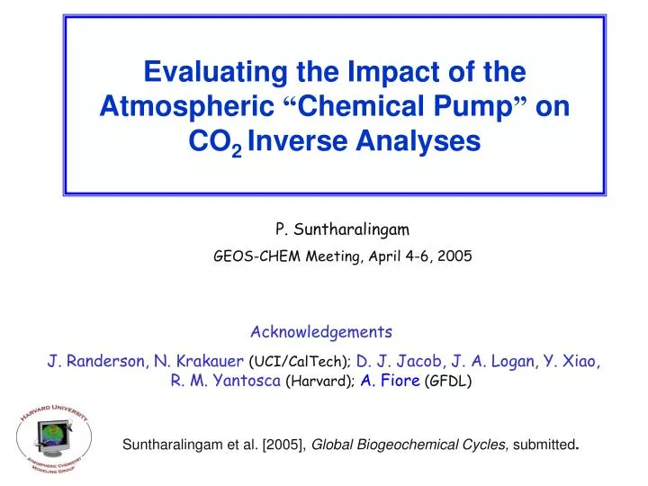
Evaluating the Impact of the Atmospheric “ Chemical Pump ” on CO 2 Inverse Analyses

1. Evaluating the Impact of the Atmospheric “Chemical Pump” on CO2 Inverse Analyses P. Suntharalingam GEOS-CHEM Meeting, April 4-6, 2005 Acknowledgements J. Randerson, N. Krakauer (UCI/CalTech); D. J. Jacob, J. A. Logan, Y. Xiao, R. M. Yantosca (Harvard); A. Fiore (GFDL) Suntharalingam et al. [2005], Global Biogeochemical Cycles, submitted.

2. APPLICATION OF GEOS-CHEM TO EVALUATE CHEMICAL PUMP EFFECT QUESTION : What is impact of accounting for realistic representation of reduced carbon oxidation 1) on modeled CO2 distributions 2) on inverse flux estimates APPROACH : Use GEOS-CHEM simulations to estimate magnitude of effect

3. ATMOSPHERIC CARBON BUDGET ? Net Terrestrial Flux ? An outstanding questionon global CO2 budget : What is magnitude and distribution of net terrestrial biospheric flux ? (“missing sink”) The “Top-down” approach usesInverse Analyses of Atmospheric CO2

4. CARBON FLUX FRAMEWORK UNDERLYING RECENT ATMOSPHERIC CO2 INVERSIONS Atmospheric CO2 Concentration residual ymod - yobs Units = Pg C/yr NET LAND UPTAKE All surface fluxes ?? ( 0-2 ) 90 6 120 92 120 “Residual Biosphere” Land use change, Fires, Regrowth, CO2 Fertilization Fossil Seasonal Biosphere Ocean

5. Inference of Northern Hemispheric Carbon Uptake from Annual Mean Concentration ResidualsTHE TRANSCOM 3 INVERSE ANALYSES (Gurney et al. 2002) Residuals = ymod– y obs Model simulations (prior fluxes) N. Hem. carbon uptake CO2 Observations • Model prior distributions for fossil, seasonal biosphere, ocean ymod • 76 Surface CO2 observation stations (GLOBALVIEW-CO2) yobs • Estimate “RESIDUAL” CO2 fluxes for 22 regions

6. OXIDATION OF REDUCED C SPECIES PROVIDES A TROPOSPHERIC SOURCE OF CO2 ATMOSPHERIC CO2 0.9-1.3 Pg C/yr Non- CO pathways Distribution of this CO2 source can be far downstream of C emission location CO NMHCs CH4 Fossil Biomass Burning, Agriculture, Biosphere Ocean

7. HOW IS REDUCED CARBON ACCOUNTED FOR IN CURRENT INVERSIONS ? A : Emitted as CO2 in surface inventories Fossil Fuel Fossil fuel : CO2 emissions based on carbon content of fuel and assuming complete oxidation of CO and volatile hydrocarbons. (Marland and Rotty, 1984; Andres et al. 1996) Seasonal Biosphere : CASA Seasonal biosphere (CASA) : Biospheric C efflux represents respiration (CO2) and emissions of reduced C gases (biogenic hydrocarbons, CH4,etc) (Randerson et al. , 2002; Randerson et al. 1997)

8. MODELING REDUCED CARBON CONTRIBUTION AT SURFACE PRODUCES BIASED INVERSION ESTIMATES ymodsurf ymod3D VS. yobs Tropospheric CO2 source from reduced C oxidation VS. Surface release of CO2 from reduced C gases CO, CH4, NMHCs Observation network detects tropospheric CO2 source from reduced C oxidation

9. CALCULATION OF CHEMICAL PUMP EFFECT yobs ymodel • Flux Estimate: x = xa+ G (y - Kxa) • STEP 1 : Impact on modeled concentrations • Adjust ymodel to account for redistribution of reduced C from surface inventories to oxidation location in troposphere • Adjustment: D ymodel = y3D –ySURF ADDeffect of CO2 source from reduced C oxidation SUBTRACTeffect of reduced C from surface inventories

10. EVALUATION OF THE CHEMICAL PUMP EFFECTGEOS-CHEM SIMULATIONS (v. 5.07) Standard Simulation CO2 Source from Reduced C Oxidation = 1.1 Pg C/yr Distribute source according to seasonal 3-D variation of CO2 production from CO Oxidation Distribute source according to seasonal SURFACE variations of reduced C emissions from Fossil and Biosphere sources CO23DSimulation : y3D CO2SURFSimulation : ySURF Simulations spun up for 3 years. Results from 4th year of simulation

11. GEOS-CHEM Model Configurationhttp://www-as.harvard.edu/chemistry/trop/geos/index.html • Global 3-D model of atmospheric chemistry (v. 5.07) • 2ox2.5o horizontal resolution; 30 vertical levels • Assimilated meteorology (GMAO); GEOS-3 (year 2001) • CO oxidation distribution from tagged CO simulation using archived monthly OH fields Reduced Carbon Emissions Distributions (spatial and temporal variability) Fossil : Duncan et al. [2005] (annual mean) Biomass Burning : Duncan et al. [2003] (monthly) Biofuels : Yevich and Logan [2003] NMVOCs : Duncan et al. [2005] ; Guenther et al. [1995]; Jacob et al. [2002] CH4 : A priori distributions from Wang et al. [2004] (monthly)

12. REDUCED CARBON SOURCES BY SECTORSTANDARD SIMULATION : CO2 Source from Reduced C Oxidation = 1.1 Pg C/yr • Sector breakdown based on Duncan et al. [2005] • *Methane sources distributed according to a priori fields from Wang et al. [2004]

13. SOURCE DISTRIBUTIONS : ANNUAL MEAN CO23D: Column Integral of CO2 from CO Oxidation CO2SURF :CO2 Emissions from Reduced C Sources gC/(cm2 yr) Zonal Integral of Emissions CO23D :Maximum in tropics, diffuse CO2SURF : Localized, corresponding to regions of high CO, CH4 and biogenic NMHC emissions CO23D CO2SURF -50 50 Latitude

14. MODELED SURFACE CONCENTRATIONS: Annual Mean CO23D CO2SURF Surface concentrations reflect source distributions: Diffuse with tropical maximum for CO23D and localized to regions of high reduced C emissions for CO2SURF

15. REGIONAL VARIATION OF CHEMICAL PUMP EFFECT Dymodel = CO23D– CO2SURF Largest changes in regions in and downstream of high reduced C emissions TAP : - 0.55; ITN : - 0.35; BAL : - 0.35 (ppm)

16. CHEMICAL PUMP EFFECT : N/S DIFFERENCES D ymodel : Zonal average at surface Mean Interhemispheric difference = - 0.21 ppm CO2 (ppm) 0.21 ppm -50 50 Latitude Impact on TRANSCOM3 Systematic decrease in Northern Hemisphere Residuals

17. IMPACT ON SURFACE FLUX ESTIMATESInverse analyses by Nir Krakauer Q :What are the changes in estimates of ‘residual’ fluxes when we account for chemical pump adjustment Dymodel Evaluate impact using TransCom annual mean analysis (Gurney et al. 2002) • Estimate effect by modifying concentration error vector as : • (y – (K xa + Dymodel)) • Then, ‘adjusted’ state estimate is: • xadj = xa + G(y – (K xa + Dymodel)) • Evaluate with 3 transport models (MATCH, GISS-UCI, LSCE-TM2)

18. REDUCTION IN LAND UPTAKE (Northern extratropics) Systematic Reduction (0.22-0.26 Pg C/year) 0.22 0.25 0.26 Pg C/yr Original Uptake 2.5 0.9 1.4 -9% -27% % Change -19% Relative impact of chemical pump adjustment on CO2 uptake varies across models.

19. SUMMARY • Neglecting the 3D representation of the CO2 source from reduced C oxidation produces biased inverse CO2 flux estimates. • Accounting for a reduced C oxidation source of 1.1 Pg C/yr gives a reduction in the modeled annual mean N-S CO2 gradient of 0.2 ppm (equivalent to a reduction of 0.2-0.3 Pg C/yr in Northern Hemispheric land uptake in an annual mean inversion.) • Regional changes are larger; up to 0.6 ppm concentration adjustment in regions of high reduced C emissions. • Impacts on seasonal inverse estimates may be significant and will be examined in future work (N/S Dy variation: –0.32 ppm (January) to –0.15 ppm (July)).

20. EXTRA SLIDES

21. SOURCE ESTIMATES FROM INVERSE ANALYSIS Minimize cost function: J(x) = (x – xa)T Sa–1 (x - xa) + (y – Kx)T Se–1 (y –K x) x = state vector (sources) xa = a priori source estimate K = Jacobian matrix (model transport) Sa = Error covariance matrix on sources Se = Error covariance matrix on concentration error Observed concentrations Modeled concentrations Solution: x = xa+ G (y - Kxa) where,G = SaKT (KSaKT + Se) -1 A posteriori errors : S= (KTSe–1K + Sa–1) -1

22. IMPACT ON SURFACE FLUX ESTIMATES Relative Reduction in N.Hemisphere Land Uptake Varies with Model Reduction in Land Uptake : MATCH Reduction in Land Uptake : LSCE-TM2

23. CHEMICAL PUMP FLUX ADJUSTMENTSZONALLY AGGREGATED LAND REGIONS Sum N. extratrop. Land net flux (PgC/yr) - 2.5 - 0.9 -1.4 Relative impact of chemical pump adjustment varies across models, though magnitude of zonally aggregated flux adjustment relatively invariant