Download
1 / 58
670 likes | 1.15k Views
Inverse Kinematics. q 4. q 5. q 2. q 3. q 1. rigid groups of atoms. T. Inverse Kinematics (IK). Given a kinematic chain (serial linkage), the position/orientation of one end relative to the other (closed chain) , find the values of the joint parameters.

E N D
q4 q5 q2 q3 q1 rigid groups of atoms T Inverse Kinematics (IK) Given a kinematic chain (serial linkage), the position/orientation of one end relative to the other (closed chain), find the values of the joint parameters
Why is IK useful for proteins? • Filling gaps in structure determination by X-ray crystallography
Automated Model Building • Software systems: RESOLVE, TEXTAL, ARP/wARP, MAID • 1.0Å < d < 2.3Å ~ 90% completeness • 2.3Å≤ d < 3.0Å ~ 67% completeness (varies widely)1 1.0Å 3.0Å JCSG: 43% of data sets 2.3Å • Manually completing a model: • Labor intensive, time consuming • Existing tools are highly interactive Model completion is high-throughput bottleneck 1Badger (2003) Acta Cryst. D59
The Completion Problem • Input: • Electron-density map • Partial structure • Two anchor residues • Amino-acid sequence of missing fragment (typically 4 – 15 residues long) • Output: • Few candidate conformation(s) of fragment that • Respect the closure constraint (IK) • Maximize match with electron-density map
Example: TM0813 PDB: 1J5X, 342 res. 2.8Å resolution 12 residue gap Best: 0.6Å aaRMSD GLU-77 GLY-90
Example: TM0813 PDB: 1J5X, 342 res. 2.8Å resolution 12 residue gap Best 0.6Å aaRMSD GLU-77 GLY-90
Why is IK useful for proteins? • Filling gaps in structure determination by X-ray crystallography • Studying the motion space of “loops” (secondary structure elements connecting a helices and b strands), which often play a key role in: • enzyme catalysis, • ligand binding (induced fit), • protein – protein interactions
Loop motion in Amylosucrase 17-residue loop that plays important role in protein’s activity
Loop 7 of 1G5A Conformations obtained by deformation sampling
Why is IK useful for proteins? • Filling gaps in structure determination by X-ray crystallography • Studying the motion space of “loops” (secondary structure elements connecting a helices and b strands), which often play a key role in: • enzyme catalysis, • ligand binding (induced fit), • protein – protein interactions • Sampling conformations using homology modeling • Chain tweaking for better prediction of folded state R. [Singh and B. Berger. ChainTweak: Sampling from the Neighbourhood of a Protein Conformation. Proc. Pacific Symposium on Biocomputing, 10:52-63, 2005.]
Generic Problem Definition • Inputs: • Protein structure with missing fragment(s) (typically 4 – 15 residues long, each) • Amino-acid sequence of each missing fragment • Outputs: • Conformation of fragment or distribution of conformations that • Respect the closure constraint (IK) • Avoid atomic clashes • Satisfy other constraints, e.g., maximize match with electron density map, minimize energy function, etc
T IK Problem • Inputs: • Closed kinematic chain with n degrees of freedom • Relative positions/orientations X of end frames • Target functionT(Q) → R • Outputs: • Conformation(s) that • Achieve closure • OptimizeT
Some Bibliographical References Biology/Crystallography • Exact IK solvers • Wedemeyer & Scheraga ’99 • Coutsias et al. ’04 • Optimization IK solvers • Fine et al. ’86 • Canutescu & Dunbrack Jr. ’03 • Ab-initio loop closure • Fiser et al. ’00 • Kolodny et al. ’03 • Database search loop closure • Jones & Thirup ’86 • Van Vlijman & Karplus ’97 • Semi-automatic tools • Jones & Kjeldgaard ’97 • Oldfield ’01 Robotics/Computer Science • Exact IK solvers • Manocha & Canny ’94 • Manocha et al. ’95 • Optimization IK solvers • Wang & Chen ’91 • Redundant manipulators • Khatib ’87 • Burdick ’89 • Motion planning for closed loops • Han & Amato ’00 • Yakey et al. ’01 • Cortes et al. ’02, ’04
Forward Kinematics q2 d2 (x,y) d1 q1 x = d1 cos q1 + d2 cos(q1+q2) y = d1sin q1+ d2 sin(q1+q2)
x2 + y2 – d12 – d22 q2 = cos-1 2d1d2 -x(d2sinq2) + y(d1 + d2cosq2) q1 = y(d2sinq2) + x(d1 + d2cosq2) Inverse Kinematics q2 d2 (x,y) d1 q1
x2 + y2 – d12 – d22 q2 = cos-1 2d1d2 -x(d2sinq2) + y(d1 + d2cosq2) q1 = y(d2sinq2) + x(d1 + d2cosq2) Inverse Kinematics d2 (x,y) d1 Two solutions
More Complicated Example q2 (x,y) d3 d2 q3 d1 q1 • Redundant linkage • Infinite number of solutions • Self-motion space
dq3 dq2 (q1,q2,q3) dq1 More Complicated Example q2 (x,y) d3 d2 q3 d1 q1 1-D space(self-motionspace)
dq3 dq2 (q1,q2,q3) dq1 More Complicated Example q2 (x,y,f) d3 d2 q3 d1 q1 • No redundancy • Finite number of solutions
General Results from Kinematics • Number of DOFs of a linkage (dimensionality of velocity space): NDOF = k(Nlink – 1) – (k–1)Njointwhere k = 3 if the linkage is planar and k = 6 if it is in 3-D space (Grübler formula, 1883). • Examples: - Open chain: Njoint = Nlink – 1 NDOF = Njoint - Closed chain: Njoint = Nlink NDOF = Njoint – k Nlink = 4 Njoint = 4NDOF = 1 Nlink = 4 Njoint = 3NDOF = 3(4-1)-(3-1)3 = 3
General Results from Kinematics • Number of DOFs of a linkage (dimension of velocity space): NDOF = k(Nlink – 1) – (k–1)Njointwhere k = 3 if the linkage is planar and k = 6 if it is in 3-D space (Grübler formula, 1883). • Examples: - Open chain: Njoint = Nlink – 1 NDOF = Njoint - Closed chain: Njoint = Nlink NDOF = Njoint – k Nlink = Njoint = NDOF = Nlink = 4 Njoint = 3NDOF = 3(4-1)-(3-1)3 = 3
General Results from Kinematics • Number of DOFs of a linkage (dimension of velocity space): NDOF = k(Nlink – 1) – (k–1)Njointwhere k = 3 if the linkage is planar and k = 6 if it is in 3-D space (Grübler formula, 1883). • Examples: - Open chain: Njoint = Nlink – 1 NDOF = Njoint - Closed chain: Njoint = Nlink NDOF = Njoint – k Nlink = 3 Njoint = 3NDOF = 0 Nlink = 4 Njoint = 3NDOF = 3(4-1)-(3-1)3 = 3
General Results from Kinematics • Number of DOFs of a linkage (dimension of velocity space): NDOF = k(Nlink – 1) – (k–1)Njointwhere k = 3 if the linkage is planar and k = 6 if it is in 3-D space (Grübler formula, 1883). • Examples: - Open chain: Njoint = Nlink – 1 NDOF = Njoint - Closed chain: Njoint = Nlink NDOF = Njoint – k 5 amino-acids10 f-y joints 10 links NDOF = 4
General Results from Kinematics 6-joint chain in 3-D space: • NDOF=0 • At most 16 distinct IK solutions
IK Methods • Analytical (exact) techniques(only for 6 joints) • Write forward kinematics in the form of polynomial equations (use t = tan(q/2) • Simplify, e.g., using the fact that two consecutive torsional angles f and y have intersecting axes [Coutsias, Seck, Jacobson, Dill, 2004] • Solve E.A. Coutsias, C. Seok, M.P. Jacobson, and K.A. Dill.A Kinematic View of Loop Closure. J. Comp. Chemistry, 25:510-528, 2004
Decomposition Method for Randomly Sampling Conformations of Closed Chains • Decompose closed chain into: • 6 “passive” joints • n-6 “active” joints
Decomposition Method for Randomly Sampling Conformations of Closed Chains • Decompose closed chain into: • 6 “passive” joints • n-6 “active” joints • Sample the active joint parameters • Compute the passive joint parameters using exact IK solver J. Cortés, T. Siméon, M. Renaud-Siméon, and V. Tran. Geometric Algorithms for the Conformational Analysis of Long Protein Loops. J. Comp. Chemistry, 25:956-967, 2004
Application of Decomposition Method Amylosucrase
IK Methods • Analytical (exact) techniques (only for 6 joints) • Write forward kinematics in the form of polynomial equations (use t = tan(q/2) • Simplify, e.g., using the fact that two consecutive torsional angles f and y have intersecting axes [Coutsias, Seck, Jacobson, Dill, 2004] • Solve • Iterative (approximate) techniques
CCD (Cyclic Coordinate Descent) Method • Generate random conformation with one end of chain at required position/orientation • Repeat until other end is at required position/orientation or algorithm is stuck at local minimum • Pick one DOF • Change to minimize closure distance L.T. Wang and C.C. Chen. A Combined Optimization Method for Solving the Inverse Kinematics Problem of Mechanical Manipulators.IEEE Tr. On Robotics and Automation, 7:489-498, 1991.
moving end fixed end Application of CCD to Proteins Closure Distance: A.A. Canutescu and R.L. Dunbrack Jr.Cyclic coordinate descent: A robotics algorithm for protein loop closure. Prot. Sci. 12:963–972, 2003. Compute and move
Example: TM0813 PDB: 1J5X, 342 res. 2.8Å resolution 12 residue gap Best: 0.6Å aaRMSD GLU-77 GLY-90
Example: TM0813 PDB: 1J5X, 342 res. 2.8Å resolution 12 residue gap Best: 0.6Å aaRMSD GLU-77 GLY-90
Advantages of CCD • Simplicity • No singularity problem • Possibility to constrain each joint independent of all others • Butmay get stuck at local minima!
CCD with Ramachandran Maps • Ramachandran maps assign probabilities to φ-ψ pairs ψ φ
CCD with Ramachandran Maps • Ramachandran maps assign probabilities to φ-ψ pairs • Change a pair (φi,ψi) at each iteration: • Compute change to φi • Compute change to ψi based on change to φi • Accept with probability min(1,Pnew/Pold)
IK Methods • Analytical (exact) techniques (only for 6 joints) • Write forward kinematics in the form of polynomial equations (use t = tan(q/2) • Simplify, e.g., using the fact that two consecutive torsional angles f and y have intersecting axes [Coutsias, Seck, Jacobson, Dill, 2004] • Solve • Iterative (approximate) techniques
Jacobian Matrix • Q: n-vector of internal coordinates • X: 6-vector defining endpoint’s position/orientation • n ≥ 6 • Forward kinematics: X = F(Q) • dxi = [∂fi(Q)/∂q1] dq1 +…+ [∂fi(Q)/∂qn] dqn • dX = J dQ Efficient algorithm to compute Jacobian:K.S. Chang and O. Khatib. Operational Space Dynamics: Efficient Algorithms for Modeling and Control of Branching Mechanisms. IEEE Int. Conf. on Robotics and Automation (ICRA),pp. 850-856, Sand Francisco, April 2000.
Jacobian Matrix J ∂f1(Q)/∂q1 ∂f1(Q)/∂q2 …∂f1(Q)/∂qn ∂f2(Q)/∂q1 ∂f2(Q)/∂q2 …∂f2(Q)/∂qn … … ∂f6(Q)/∂q1 ∂f6(Q)/∂q2 …∂f6(Q)/∂qn
Case where n = 6 • J is a square 6x6 matrix. • Problem: Given X, find Q such that X= F(Q) • Start at any X0 = F(Q0) • Method: • Interpolate linearly between X0 and X sequence X1, X2, …, Xp = X • For i = 1,…,p do • Qi = Qi-1 + J-1(Qi-1)(Xi-Xi-1) • Reset Xi to F(Qi)
Case where n > 6 • dX = J dQ • J is an 6n matrix. Assume rank(J) = 6. • Null space { dQ0 | J dQ0 = 0} has dim = n - 6
arbitrarily chosenin null space Case where n > 6 • dX = J dQ • J is an 6n matrix. Assume rank(J) = 6 • Find J+ (pseudo-inverse) such that JJ+ = I dQ = J+dX • Null space { dQ0 | J dQ0 = 0} has dim = n - 6 • dQ = J+dX + dQ0
s1 s2 0 s6 Computation of J+ • SVD decomposition J = U S VT where: - U in an 66 square orthonormal matrix- V is an n6 square orthonormal matrix- S is of the form diag[si]: • J+ = V S+ UT where S+=diag[1/si]
Getting Null space J S66 dX U66 VT6n dQ =
Getting Null space J S6n dX U66 VTnn dQ 0 = Gram-Schmidt orthogonalization