Download
1 / 34
580 likes | 2.73k Views
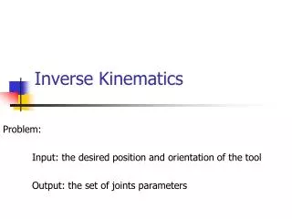
Introduction to ROBOTICS. Inverse Kinematics Jacobian Matrix Trajectory Planning . Dr. Jizhong Xiao Department of Electrical Engineering City College of New York jxiao@ccny.cuny.edu. Outline. Review Kinematics Model Inverse Kinematics Example Jacobian Matrix Singularity

E N D
Introduction to ROBOTICS Inverse KinematicsJacobian MatrixTrajectory Planning Dr. Jizhong Xiao Department of Electrical Engineering City College of New York jxiao@ccny.cuny.edu
Outline • Review • Kinematics Model • Inverse Kinematics • Example • Jacobian Matrix • Singularity • Trajectory Planning
Review • Steps to derive kinematics model: • Assign D-H coordinates frames • Find link parameters • Transformation matrices of adjacent joints • Calculate kinematics matrix • When necessary, Euler angle representation
Denavit-Hartenberg Convention • Number the joints from 1 to n starting with the base and ending with the end-effector. • Establish the base coordinate system. Establish a right-handed orthonormal coordinate system at the supporting base with axis lying along the axis of motion of joint 1. • Establish joint axis. Align the Zi with the axis of motion (rotary or sliding) of joint i+1. • Establish the origin of the ith coordinate system. Locate the origin of the ith coordinate at the intersection of the Zi & Zi-1 or at the intersection of common normal between the Zi & Zi-1 axes and the Zi axis. • Establish Xi axis. Establish or along the common normal between the Zi-1 & Zi axes when they are parallel. • Establish Yi axis. Assign to complete the right-handed coordinate system. • Find the link and joint parameters
Review • Link and Joint Parameters • Joint angle : the angle of rotation from the Xi-1 axis to the Xi axis about the Zi-1 axis. It is the joint variable if joint i is rotary. • Joint distance : the distance from the origin of the (i-1) coordinate system to the intersection of the Zi-1 axis and the Xi axis along the Zi-1 axis. It is the joint variable if joint i is prismatic. • Link length : the distance from the intersection of the Zi-1 axis and the Xi axis to the origin of the ith coordinate system along the Xi axis. • Link twist angle : the angle of rotation from the Zi-1 axis to the Zi axis about the Xi axis.
Review • D-H transformation matrix for adjacent coordinate frames, i and i-1. • The position and orientation of the i-th frame coordinate can be expressed in the (i-1)th frame by the following 4 successive elementary transformations: Source coordinate Reference Coordinate
Review • Kinematics Equations • chain product of successive coordinate transformation matrices of • specifies the location of the n-th coordinate frame w.r.t. the base coordinate system Orientation matrix Position vector
Review • Kinematics Transformation • Matrix • Forward Kinematics Why use Euler angle representation? What is ?
Review • Yaw-Pitch-Roll Representation (Equation A)
Review • Compare LHS and RHS of Equation A, we have:
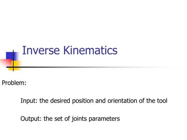
Inverse Kinematics • Transformation Matrix • Robot dependent, Solutions not unique • Systematic closed-form solution in general is not available • Special cases make the closed-form arm solution possible: • Three adjacent joint axes intersecting (PUMA, Stanford) • Three adjacent joint axes parallel to one another (MINIMOVER)
Example • Solving the inverse kinematics of Stanford arm
Example • Solving the inverse kinematics of Stanford arm Equation (1) Equation (2) Equation (3) In Equ. (1), let
Example • Solving the inverse kinematics of Stanford arm From term (3,3) From term (1,3), (2,3)
Example • Solving the inverse kinematics of Stanford arm
Jacobian Matrix Forward Jacobian Matrix Kinematics Inverse Jacobian Matrix: Relationship between joint space velocity with task space velocity Joint Space Task Space
Jacobian Matrix Forward kinematics
Jacobian Matrix Jacobian is a function of q, it is not a constant!
Jacobian Matrix Forward Kinematics Linear velocity Angular velocity
(x , y) - 2 l2 l1 1 Example • 2-DOF planar robot arm • Given l1, l2 ,Find: Jacobian
Jacobian Matrix • Physical Interpretation How each individual joint space velocity contribute to task space velocity.
Jacobian Matrix • Inverse Jacobian • Singularity • rank(J)<min{6,n}, Jacobian Matrix is less than full rank • Jacobian is non-invertable • Boundary Singularities: occur when the tool tip is on the surface of the work envelop. • Interior Singularities: occur inside the work envelope when two or more of the axes of the robot form a straight line, i.e., collinear
V (x , y) l2 Y 2 =0 l1 1 x Quiz • Find the singularity configuration of the 2-DOF planar robot arm determinant(J)=0 Not full rank Det(J)=0
Jacobian Matrix • Pseudoinverse • Let A be an mxn matrix, and let be the pseudoinverse of A. If A is of full rank, then can be computed as: • Example:
Robot Motion Planning • Path planning • Geometric path • Issues: obstacle avoidance, shortest path • Trajectory planning, • “interpolate” or “approximate” the desired path by a class of polynomial functions and generates a sequence of time-based “control set points” for the control of manipulator from the initial configuration to its destination.
Trajectory planning • Path Profile • Velocity Profile • Acceleration Profile
The boundary conditions 1) Initial position 2) Initial velocity 3) Initial acceleration 4) Lift-off position 5) Continuity in position at t1 6) Continuity in velocity at t1 7) Continuity in acceleration at t1 8) Set-down position 9) Continuity in position at t2 10) Continuity in velocity at t2 11) Continuity in acceleration at t2 12) Final position 13) Final velocity 14) Final acceleration
Requirements • Initial Position • Position (given) • Velocity (given, normally zero) • Acceleration (given, normally zero) • Final Position • Position (given) • Velocity (given, normally zero) • Acceleration (given, normally zero)
Requirements • Intermediate positions • set-down position (given) • set-down position (continuous with previous trajectory segment) • Velocity (continuous with previous trajectory segment) • Acceleration (continuous with previous trajectory segment)
Requirements • Intermediate positions • Lift-off position (given) • Lift-off position (continuous with previous trajectory segment) • Velocity (continuous with previous trajectory segment) • Acceleration (continuous with previous trajectory segment)
Trajectory Planning • n-th order polynomial, must satisfy 14 conditions, • 13-th order polynomial • 4-3-4 trajectory • 3-5-3 trajectory t0t1, 5 unknow t1t2, 4 unknow t2tf, 5 unknow
How to solve the parameters • Handout in the class
Thank you! Homework 3 posted on the web. Next class: Robot Dynamics