Download
1 / 33
2.34k likes | 6.63k Views
Ch. 3: Forward and Inverse Kinematics. Recap: The Denavit-Hartenberg (DH) Convention. Representing each individual homogeneous transformation as the product of four basic transformations:. 03_03. Recap: the physical basis for DH parameters.

E N D
Ch. 3: Forward and Inverse Kinematics ES159/259
Recap: The Denavit-Hartenberg (DH) Convention • Representing each individual homogeneous transformation as the product of four basic transformations: ES159/259
03_03 Recap: the physical basis for DH parameters • ai: link length, distance between the o0 and o1 (projected along x1) • ai: link twist, angle between z0 and z1 (measured around x1) • di: link offset, distance between o0 and o1 (projected along z0) • qi: joint angle, angle between x0 and x1 (measured around z0) ES159/259
General procedure for determining forward kinematics • Label joint axes as z0, …, zn-1 (axis zi is joint axis for joint i+1) • Choose base frame: set o0 on z0 and choose x0 and y0 using right-handed convention • For i=1:n-1, • Place oi where the normal to zi and zi-1 intersects zi. If zi intersects zi-1, put oi at intersection. If zi and zi-1 are parallel, place oi along zi such that di=0 • xi is the common normal through oi, or normal to the plane formed by zi-1 and zi if the two intersect • Determine yi using right-handed convention • Place the tool frame: set zn parallel to zn-1 • For i=1:n, fill in the table of DH parameters • Form homogeneous transformation matrices, Ai • Create Tn0 that gives the position and orientation of the end-effector in the inertial frame ES159/259
03_02tbl Example 2: three-link cylindrical robot • 3DOF: need to assign four coordinate frames • Choose z0 axis (axis of rotation for joint 1, base frame) • Choose z1 axis (axis of translation for joint 2) • Choose z2 axis (axis of translation for joint 3) • Choose z3 axis (tool frame) • This is again arbitrary for this case since we have described no wrist/gripper • Instead, define z3 as parallel to z2 ES159/259
03_02tbl Example 2: three-link cylindrical robot • Now define DH parameters • First, define the constant parameters ai, ai • Second, define the variable parameters qi, di ES159/259
03_03tbl Example 3: spherical wrist • 3DOF: need to assign four coordinate frames • yaw, pitch, roll (q4, q5, q6) all intersecting at one point o (wrist center) • Choose z3 axis (axis of rotation for joint 4) • Choose z4 axis (axis of rotation for joint 5) • Choose z5 axis (axis of rotation for joint 6) • Choose tool frame: • z6 (a) is collinear with z5 • y6 (s) is in the direction the gripper closes • x6 (n) is chosen with a right-handed convention ES159/259
03_03tbl Example 3: spherical wrist • Now define DH parameters • First, define the constant parameters ai, ai • Second, define the variable parameters qi, di ES159/259
03_09 Example 4: cylindrical robot with spherical wrist • 6DOF: need to assign seven coordinate frames • But we already did this for the previous two examples, so we can fill in the table of DH parameters: o3, o4, o5 are all at the same point oc ES159/259
03_09 Example 4: cylindrical robot with spherical wrist • Note that z3 (axis for joint 4) is collinear with z2 (axis for joint 3), thus we can make the following combination: ES159/259
03_10 Example 5: the Stanford manipulator • 6DOF: need to assign seven coordinate frames: • Choose z0 axis (axis of rotation for joint 1, base frame) • Choose z1-z5 axes (axes of rotation/translation for joints 2-6) • Choose xi axes • Choose tool frame • Fill in table of DH parameters: Suggested insertion: photo of the Stanford manipulator ES159/259
03_04tbl Example 5: the Stanford manipulator • Now determine the individual homogeneous transformations: ES159/259
03_04tbl Example 5: the Stanford manipulator • Finally, combine to give the complete description of the forward kinematics: ES159/259
03_11 Example 6: the SCARA manipulator • 4DOF: need to assign five coordinate frames: • Choose z0 axis (axis of rotation for joint 1, base frame) • Choose z1-z3 axes (axes of rotation/translation for joints 2-4) • Choose xi axes • Choose tool frame • Fill in table of DH parameters: Suggested insertion: photo of SCARA manipulator ES159/259
03_04tbl Example 6: the SCARA manipulator • Now determine the individual homogeneous transformations: ES159/259
Forward kinematics of parallel manipulators • Parallel manipulator: two or more series chains connect the end-effector to the base (closed-chain) • # of DOF for a parallel manipulator determined by taking the total DOFs for all links and subtracting the number of constraints imposed by the closed-chain configuration • Gruebler’s formula (3D): #DOF for joint i number of links* number of joints ES159/259 *excluding ground
Forward kinematics of parallel manipulators • Gruebler’s formula (2D): • Example (2D): • Planar four-bar, nL = 3, nj = 4, fi = 1(for all joints) • 3(3-4)+4 = 1DOF • Forward kinematics: ES159/259
Inverse Kinematics • Find the values of joint parameters that will put the tool frame at a desired position and orientation (within the workspace) • Given H: • Find all solutions to: • Noting that: • This gives 12 (nontrivial) equations with n unknowns ES159/259
Example: the Stanford manipulator • For a given H: • Find q1, q2, d3, q4, q5, q6: • One solution: q1 = p/2, q2 = p/2, d3 = 0.5, q4 = p/2, q5 = 0, q6 = p/2 ES159/259
Inverse Kinematics • The previous example shows how difficult it would be to obtain a closed-form solution to the 12 equations • Instead, we develop systematic methods based upon the manipulator configuration • For the forward kinematics there is always a unique solution • Potentially complex nonlinear functions • The inverse kinematics may or may not have a solution • Solutions may or may not be unique • Solutions may violate joint limits • Closed-form solutions are ideal! ES159/259
03_12 Overview: kinematic decoupling • Appropriate for systems that have an arm a wrist • Such that the wrist joint axes are aligned at a point • For such systems, we can split the inverse kinematics problem into two parts: • Inverse position kinematics: position of the wrist center • Inverse orientation kinematics: orientation of the wrist • First, assume 6DOF, the last three intersecting at oc • Use the position of the wrist center to determine the first three joint angles… ES159/259
03_12 Overview: kinematic decoupling • Now, origin of tool frame, o6, is a distance d6 translated along z5 (since z5 and z6 are collinear) • Thus, the third column of R is the direction of z6 (w/ respect to the base frame) and we can write: • Rearranging: • Calling o = [oxoyoz]T, oc0 = [xcyczc]T ES159/259
03_12 Overview: kinematic decoupling • Since [xcyczc]T are determined from the first three joint angles, our forward kinematics expression now allows us to solve for the first three joint angles decoupled from the final three. • Thus we now have R30 • Note that: • To solve for the final three joint angles: • Since the last three joints for a • spherical wrist, we can use a set of • Euler angles to solve for them ES159/259
03_13 Inverse position • Now that we have [xcyczc]T we need to find q1, q2, q3 • Solve for qi by projecting onto the xi-1, yi-1 plane, solve trig problem • Two examples: elbow (RRR) and spherical (RRP) manipulators • For example, for an elbow manipulator, to solve for q1, project the arm onto the x0, y0 plane ES159/259
Background: two argument atan • We use atan2(·) instead of atan(·) to account for the full range of angular solutions • Called ‘four-quadrant’ arctan ES159/259
03_14 Example: RRR manipulator • To solve for q1, project the arm onto the x0, y0 plane • Can also have: • This will of course change the solutions for q2 and q3 ES159/259
If there is an offset, then we will have two solutions for q1: left arm and right arm However, wrist centers cannot intersect z0 If xc=yc=0, q1 is undefined i.e. any value of q1 will work 03_15 Caveats: singular configurations, offsets ES159/259
Left arm: Right arm: 03_17 Left arm and right arm solutions ES159/259
03_19 Left arm and right arm solutions • Therefore there are in general two solutions for q1 • Finding q2 and q3 is identical to the planar two-link manipulator we have seen previously: • Therefore we can find two solutions for q3: ES159/259
03_19 Left arm and right arm solutions • The two solutions for q3 correspond to the elbow-down and elbow-up positions respectively • Now solve for q2: • Thus there are two solutions for the pair (q2, q3) ES159/259
03_20 RRR: Four total solutions • In general, there will be a maximum of four solutions to the inverse position kinematics of an elbow manipulator • Ex: PUMA ES159/259
03_21 Example: RRP manipulator • Spherical configuration • Solve for q1 using same method as with RRR • Again, if there is an offset, there will be left-arm and right-arm solutions • Solve for q2: • Solve for d3: ES159/259
Next class… • Complete the discussion of inverse kinematics • Inverse orientation • Introduction to other methods • Introduction to velocity kinematics and the Jacobian ES159/259