Download
1 / 20
210 likes | 565 Views
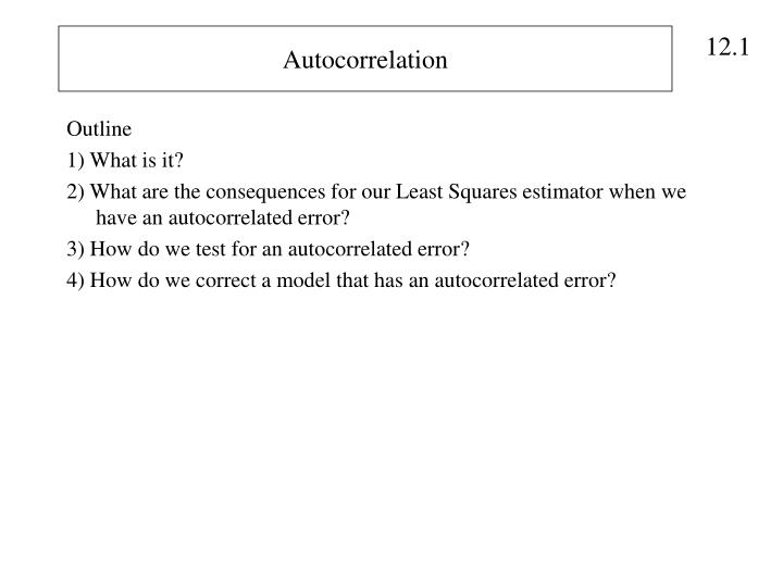
Autocorrelation. Outline 1) What is it? 2) What are the consequences for our Least Squares estimator when we have an autocorrelated error? 3) How do we test for an autocorrelated error? 4) How do we correct a model that has an autocorrelated error?. What is Autocorrelation?.

E N D
Autocorrelation Outline 1) What is it? 2) What are the consequences for our Least Squares estimator when we have an autocorrelated error? 3) How do we test for an autocorrelated error? 4) How do we correct a model that has an autocorrelated error?
What is Autocorrelation? Review the assumption of Gauss-Markov • Linear Regression Model y = 1 + 2x + e • Error Term has a mean of zero: E(e) = 0 E(y) = 1 + 2x • Error term has constant variance: Var(e) = E(e2) = 2 • Error term is not correlated with itself (no serial correlation): Cov(ei,ej) = E(eiej) = 0 ij • Data on X are not random and thus are uncorrelated with the error term: Cov(X,e) = E(Xe) = 0 This is the assumption of a serially uncorrelated error. The error is assumed to be independent of its past; it has no memory of its past values. It is like flipping a coin. A a serial correlated error (a.k.a. autocorrelated error) is one that has a memory of its past values. It is correlated with itself. Autocorrelation is more commonly a problem for time-series data.
An example of an autocorrelated error: Here we have = 0.8. It means that 80% of the error in period t-1 is still felt in period t. The error in period t is comprised of 80% of last period’s error plus an error that is unique to period t. This is sometimes called an AR(1) model for “autoregressive of the first order” The autocorrelation coefficient must lie between –1 and 1: -1 < < 1 Anything outside this range is unstable and very unlikely for economic models
Autocorrelation can be positive or negative: if > 0 we say that the error has positive autocorrelation. A graph of the errors shows a tracking pattern: if < 0 we say that the error has negative autocorrelation. A graph of the errors shows an oscillating pattern: • In general measures the strength of the correlation between the errors at time t and their values lagged one period. • There can be higher orders such as a second order AR(2) model:
What are the Implications for Least Squares? We have to ask “where did we used the assumption”? Or “why was the assumption needed in the first place?” We used the assumption in the derivation of the variance formulas for the least squares estimators, b1 and b2. For b2 this was The assumption of a serially uncorrelated error is made when we say that the variance of a sum is equal to the sum of the variances. This is true only if the random variables are uncorrelated. See Chapter 2, pg. 31.
The proof that the least squares estimators is unbiased did not use the assumption of serially uncorrelated errors; therefore, this property of least squares continues to hold even in the presence of a autocorrelated error. • The “B” in BLUE of the Gauss-Markov Theorem no longer holds. • The variance formulas for the least squares estimators are incorrect invalidates hypoth tests and confidence intervals. The “correct” variance formula: The large term in brackets shows how the Var(b2) formula changes to allow for an autocorrelated error.
If > 0 which is typically the case for economic models, it can be shown that the “incorrect” Var(b2) < “correct” Var(b2). • If we ignore the problem and use the “incorrect” Var(b2) we will overstate the reliability of the estimates, because we will report a standard error that is too small. The t-statistics will be “falsely” large, leading to a false sense of precision.
How to Test for Autocorrelation We test for autocorrelation similar to how we test for a heteroskedastic error: estimate the model using least squares and examine the residuals for a pattern. • Visual Inspection: Plot residuals against time. Do they have a systematic pattern that indicates a tracking pattern (for positive autocorrelation) or an oscillating pattern (for negative autocorrelation)? Example: a model of Job Vacancies and the Unemployment Rate Page 278, Exercise 12.3 ln(JV)t = 1 + 2 ln(U)t + et Where JV are job vacancies, U is the unemployment rate.
Sum of Mean Source DF Squares Square F Value Pr > F Model 1 8.72001 8.72001 107.36 <.0001 Error 22 1.78687 0.08122 Corrected Total 23 10.50688 Root MSE 0.28499 R-Square 0.8299 Dependent Mean 0.63427 Adj R-Sq 0.8222 Coeff Var 44.93266 Parameter Estimates Parameter Standard Variable DF Estimate Error t Value Pr > |t| Intercept 1 3.50270 0.28288 12.38 <.0001 lu 1 -1.61159 0.15554 -10.36 <.0001 ^ ln(JV)t = 3.503 – 1.612 ln(U)t
2) Formal Test: Durbin-Watson Test This test is based on the residuals from the least squares regression. (remember that our test for heteroskedasticity was also based on the residuals from a least squares regression) If the error term has first-order serial correlation, et = et-1 + vt • The residuals at t and t-1 ought to be correlated. Ho: = 0 H1: > 0 (positive autocorrelation is more likely in economics) The Durbin-Watson test statistic is used to test this hypothesis. It is constructed using the least squares residuals. Specifically:
The d statistic can be simplified into an expression involving The sample correlation between the residuals at t and t-1: ^ ^ Note that if there is no autocorrelation, then = 0, so that should also be around 0, implying a d-statistic of 2. If = 1 d = 0 If = -1 d = 4 The question then becomes: “How far below 2 must the d-statistic be to say that there is positive autocorrelation?” and “How far above 2 must the d-statistic be to say that there is negative autocorrelation?”
Typically we want to compare our test statistic to a critical value to determine whether or not the data reject the null hypothesis. The probability distribution for the d-statistic have some convenient well-known form such as the t or the F. Instead, its distribution depends on the values of the explanatory variables. For this reason, the best we can do is tie down a lower and upper bound for the critical d values. See Table 5, pg 393-396. Suppose T=24 observations used to estimate a model with one independent variable and an intercept k = 2. 1) The test: Ho: = 0 H1: > 0 2) Calculate the d-statistic according to the formula on slide 12.11 Conduct the test If d < 1.273 reject Ho If d > 1.446 fail to reject Ho If 1.273 < d < 1.446 inconclusive 2 0 dL 1.273 dU 1.446 4 d
Example: Test the model of job vacancies. For this model T=24, and k=2 we can use the dL and dU critical values from slide 12.13. To calculate the durbin-watson d-statistic, we get SAS to do so by adding the dw option to the model statement: Proc reg; model ljv = lu / dw; Run; The REG Procedure Model: MODEL1 Dependent Variable: ljv Durbin-Watson D 1.090 Number of Observations 24 1st Order Autocorrelation 0.432 Conclusion: reject Ho because d = 1.09 < 1.273
How to Correct for Autocorrelation • It is quite possible that the error in a regression equation appears to be autocorrelated due to an omitted variable. Recall that omitted variables “end up” in the error term. If the omitted variable is correlated over time (which is true of many economic time-series), then the residuals will appear to track Correct the problem by reformulating the model (include the omitted variable) 2) Generalized Least Squares Similar to the problem of a heteroskedastic error, we will take our model that has an autocorrelated error and transform it into a model that has a well-behaved (serially uncorrelated) error.
The original model: where: vt is a “well-behaved” error that is serially uncorrelated Algebraic manipulations:
Construct new variables: These variables are sometimes called “generalized differences”. We will then estimate this model using the new variables: Note that x1* is really a constant, not a variable. The intercept 1 has always been multiplied by 1 and now it is multiplied by (1-)
The problem is, what to use for because it is unknown? • There are many different ways of estimating . • All methods begin with the residuals from least squares, • the same residuals used to construct the durbin-watson test statistic: • 2) Use this estimate of to construct the generalized differences • according to the formulas on the previous slide for y*, x1* and x2* • 3) Run Least Squares using these generalized differences • 4) (Cochrane-Orcutt’s Iterative Procedure) [a.k.a Yule-Walker Method] • From step 3), take the residuals from this regression • and repeat steps 1) – 3). Each time you get new estimates of 1 and 2. • Continue to iterative until the values of the estimates converge.
The AUTOREG Procedure Dependent Variable ljv Ordinary Least Squares Estimates SSE 1.78686627 DFE 22 MSE 0.08122 Root MSE 0.28499 SBC 12.1229868 AIC 9.76687918 Regress R-Square 0.8299 Total R-Square 0.8299 Durbin-Watson 1.0896 Standard Approx Variable DF Estimate Error t Value Pr > |t| Intercept 1 3.5027 0.2829 12.38 <.0001 lu 1 -1.6116 0.1555 -10.36 <.0001 Estimates of Autocorrelations Lag Covariance Correlation -1 9 8 7 6 5 4 3 2 1 0 1 2 3 4 5 6 7 8 9 1 0 0.0745 1.000000 | |********************| 1 0.0322 0.431840 | |********* | Preliminary MSE 0.0606 Estimates of Autoregressive Parameters Standard Lag Coefficient Error t Value 1 -0.431840 0.196822 -2.19 Yule-Walker Estimates SSE 1.4379184 DFE 21 MSE 0.06847 Root MSE 0.26167 SBC 10.2930273 AIC 6.75886582 Regress R-Square 0.8853 Total R-Square 0.8631 Durbin-Watson 2.0166 The AUTOREG Procedure Standard Approx Variable DF Estimate Error t Value Pr > |t| Intercept 1 3.5138 0.2437 14.42 <.0001 lu 1 -1.6162 0.1269 -12.73 <.0001 These results will be discussed in class.
options ls=78; options formdlim='*'; goptions reset=all; data one; infile 'c:\my documents\classes\UE\datafiles\vacan.dat' firstobs=2; input jv u; time=_n_; ljv = log(jv); lu = log(u); symbol1 i=none c=red v=dot h=.5; symbol2 c=black i=join l=1; proc gplot ; plot ljv * lu = 1 ; proc autoreg; model ljv = lu / dwprob; output out=stuff residual= ehat predicted=ljv_hat; run; proc gplot data=stuff; plot ljv*mortg=1 ljv_hat*mortg = 2 / overlay legend; plot ehat*time=1 / vref=0; proc autoreg; model ljv = lu / nlag=1; run; use PROC AUTOREG with DWPROB to get p-values for the DW statistic Using PROC AUTOREG with the / nlag=1 option in the model statement will estimate the model and correct for first-order autocorrelation in the errors.