Download
1 / 28
280 likes | 292 Views
SIMPLE MODELS OF HELICAL BAROCLINIC VORTICES. Michael V. Kurgansky A.M. Obukhov Institute of Atmospheric Physics, Moscow – RUSSIA E-mail: kurgansk@ifaran.ru. Workshop TODW01 “Topological Fluid Dynamics (IUTAM Symposium) “ Isaac Newton Institute for Mathematical Sciences

E N D
SIMPLE MODELS OF HELICAL BAROCLINIC VORTICES Michael V. Kurgansky A.M. Obukhov Institute of Atmospheric Physics, Moscow – RUSSIA E-mail: kurgansk@ifaran.ru Workshop TODW01 “Topological Fluid Dynamics (IUTAM Symposium) “ Isaac Newton Institute for Mathematical Sciences Cambridge, UK, July 23-27, 2012
OUTLINE: 1.Introduction/Motivation. •Applications to the dynamics of tornadoes and dust devils •Generalization of the Rankine vortex model (with a core axial flow) onto the case of fluid baroclinicity, under Boussinesq approximation (for an axially directed buoyancy force confined to the vortex core) •Construction of as simple as possible vortex models, which provide such a generalization 2. Self-similar vortex solution •Preliminaries and basics •Controlling role of the vortex breakdown 3. A ´vortical cone´ model •General formulation •Helicity budget 4. Magneto-hydrostatic analogy SUMMARY/CONCLUSIONS
A tornado near Anadarko, Oklahoma on May 3, 1999 (VORTEX 99; Verification of the Origins of Rotation in Tornadoes Experiment ) A dust devil in the Atacama Desert near Huara, Chile (January 2009) Two characteristic morphological forms of dust devils: (a) rope-type vortices and (b) vase-type vortices
‘Demon spawn’ (I) A large, poorly structured dust-laden column is accompanied with a tightly-organized, small ‘tube’ column at the leading edge of the advancing system. The smaller column rotated in the counter direction to the main vortex and it wrapped around the larger column. By placing the chase truck between them the delicately balanced air-flow was disrupted and the smaller vortex was dissipated [see Metzger S, Kurgansky M, Montecinos A, Villagran V, Verdejo H, ”Chasing dust devils in Chile’s Atacama Desert”, Lunar & Planetary Science Conference, Houston, USA, March 2010].
‘Demon spawn’ (II) A large, poorly structured dust-laden column is accompanied with a tightly-organized, small ‘tube’ column at the leading edge of the advancing system. The smaller column rotated in the counter direction to the main vortex and it wrapped around the larger column. By placing the chase truck between them the delicately balanced air-flow was disrupted and the smaller vortex was dissipated [see Metzger S, Kurgansky M, Montecinos A, Villagran V, Verdejo H, ”Chasing dust devils in Chile’s Atacama Desert”, Lunar & Planetary Science Conference, Houston, USA, March 2010].
Preliminaries Momentum balance and mass continuity equations for a weakly compressible airflow (under the Boussinesq approximation) in an inertial reference frame read Here, v is the velocity, the non-hydrostatic pressure divided by an average air density, b the buoyancy force, and F the turbulent viscous force. In polar cylindrical (r,,z) - coordinates, two integral formulas follow from the non-linear thermal wind equation for a steady axisymmetricinviscid flow: (1) (2) Here, b is the buoyancy; v (u,v,w) and (r,,z) are the velocity and the vorticity vectors; z and z are two arbitrary altitudinal levels.
General equation of balance of helicity in a Boussinesq fluid : Here, b is the buoyancy force and F is the turbulent viscous force; S denotes the helicity flux vector. For a steady axisymmetricinviscid flow this general balance equation (Kurgansky, 2008) is equivalent to Eq. (2).
Self-similar vortex solution (helical baroclinicRankine-like vortex #1): The similarity assumptions are used when the relative distribution of velocity components is the same across the vortex at all altitudes. The rotational velocity v at each horizontal level has a profile which is characteristic for a Rankine vortex with irrotational flow periphery (cf. Kelvin Lord, 1880). The vertical velocity w in the vortex core corresponds to an updraft flow. At each horizontal level w is uniform inside the vortex core; in the peripheral flow w. The radius of the vortex core rmz is a monotonic increasing function of altitude z. A non-linear differential equation (Kurgansky, 2005; cf. a magnetostatic problem for sunspots inSchlüter and Temesváry, 1958) follows from Eq. (1) and describes the vortex constitution, given the specific angular momentum and the vertical volumetric flux Q, and provided bz were prescribed. The morphologically simplest vortex solution reads (Kurgansky, 2005)
Self-similar vortex solution (helical baroclinicRankine-like vortex #1) (a) FIGURE 1. Schematic of helical baroclinic Rankine vortex #1
The singular level z h is associated with the top of atmospheric convective boundary layer; the earth surface is at z . The vortex solution is valid beginning with a critical height z h, where the vortex breakdown occurs. If applied to the level z , it yields (3) The helical parameter w vmis the reciprocal of the ‘swirl ratio’; Eq. (3) for the maximum wind speed vm is reminiscent of the ‘thermodynamical speed limit’ but contains an important dependence on -parameter. Controllingaction of thevortexbreakdown (Benjamin, 1962; Leibovich, 1970; Fiedler & Rotunno, 1986, and others) impliesthat orequivalently Fortheprescibed ´buoyantmoment´, b(0, ) ( h )const , thevortexisstrongestwhentheRankine-likeswirlingconvectiveplumewithinthesurfaceadjacentlayer z isleastsupercritical; compare withthemaximumefficiency of an ideal (reversible) Carnot´sheatengine.
Vortex breakdown The vertical momentum flux constancy across the breakdown level Two conjugate states (supercritical and subcritical) exist when (cf. Fiedler and Rotunno, 1987) A critical value for the vortex breakdown The vertical energy flux experiences a negative jump across the breakdown level (X2>X1)
A ´vortical cone´ model (helical baroclinicRankine vortex #2) A swirling (warm) buoyant plume with irrotationalpoloidal flow component (u,w) is ejected from a ‘virtual’ source of mass, which is located beneath the earth surface at z d (cf. Morton et al., 1956). The radius of the vortex core linearly increases with height The azimuthal component of vorticity has - singularity at the plume edge and and identically vanishes elsewhere. The rotational velocity v at each horizontal level has the same profile as in helical baroclinicRankine vortex #1; the vortex core is congruent to the plume. The vortex solution has a physical meaning at z ( d).For this slender vortex and in full conformity with Eq. (3), Eq. (1) gives at z : (4) All arguments [concerning the vortex breakdown and subsequent vortex truncation at z ] that are relevant to Eq. (3) equally apply to Eq. (4).
A ´vortical cone´ model (helical baroclinicRankine-like vortex #2) (b) FIGURE 2. Schematic of helical baroclinic Rankine vortex #2
Downward helicity flux For helical baroclinicRankine vortex #2 the downward helicity flux S across the vortex breakdown (vortex truncation) level, z , reads [O(c2)) terms are neglected)] (5) With good accuracy Eq. (5) is applicable to helical baroclinicRankine vortex #1; a minor discrepancy results from a weak artificial upward flux of the helicity across the singular level zh which adds to (5) and manifests itself at all altitudes including zh . For a slenderhelicalbaroclinicRankinevortexthe vertical energy flux Jzisproportionaltothe vertical helicity flux Sz:
Helicity budget FIGURE 3. Sketch of the helicity budget in helical baroclinicRankine Vortex #2 (not in scale)
Total helicity of the vortex flow Helical baroclinicRankine vortex #2 possesses a well-defined finite total helicity value which is equal to the doubled product of the toroidalKtvmrmand the poloidalKpvmd Kelvin’s velocity circulation (cf. Moffatt, 1969). For helical baroclinicRankine vortex #1, the total helicityH is infinite , due to an increasingly growing contribution from v –product when zh.
Magneto-hydrostatic analogues to ´dual´ helical baroclinicRankine-like vortices ##1,2 Self-similar approachwithin a magneto-hydrostaticproblemfor a ´magnetichole´ (compare, Schlüterand Temesváry, 1958); is the magnetic permeability and pethe (reference) atmospheric pressure: The first and the second left-hand side terms describe the magnetic tension and magnetic pressure, respectively, both due to the poloidal magnetic field component. The third term describes the magnetic tension effect from the twist (toroidal) magnetic field component; it is neglected hereafter, like in Schlüter and Temesváry (1958). Polytropic reference atmosphere: Two alternative cases (depending on - sign): A B
Magneto-hydrostatic analogues to ´dual´ helical baroclinicRankine vortices ##1,2 Two particular cases: For a solar ionized (monoatomic) atmosphere: I Magnetic tension vanishes => an analogue of helical baroclinicRankine-like vortex #1 II Magnetic tension term does not vanish, as in the previous case, but is proportional to the dominating magnetic pressure term => an analogue of helical baroclinicRankine-like vortex #2 A duality between two Rankine-like helical baroclinic vortices exists, the first one being the simplest examle of such a vortex and the second one being the next to the simplest.
Summary/Conclusions • Two distinct asymptotic solutions of inviscidBoussinesq equations for a steady helical baroclinicRankine-like vortex with prescribed buoyant forcing are considered and critically compared. In both cases the relative distribution of the velocity components is the same across the vortex at all altitudes (the similarity assumption). The first vortex solution demonstrates monotonic growth with height of the vortex core radius, which becomes infinite at a certain critical altitude, and the corresponding attenuation of the vertical vorticity. The second vortex solution schematizes the vortex core as an inverted cone of small angular aperture. • The idealized vortices are embedded in a convectively unstable boundary layer: the inviscid asymptotic solution are truncated at a small height over the ground at which the vortex breakdown takes place. • Both models predict essentially the same dependence of the model-inferred peak rotational velocity on the swirl number (the ratio of the maximum swirl velocity to the average vertical velocity in the main vortex updraft). • The helicity budget for the second vortex solution has been successfully balanced, whereas for the first vortex solution this analysis would meet certain difficulties due to the model singularity at a critical level.
References • Kelvin Lord (1880) Phil Mag 10: 155-168 • Barcilon A (1967) J Fluid Mech 27: 155-175 • Benjamin TB (1962) J Fluid Mech 14: 593-629 • Fiedler BH, Rotunno R (1986) J AtmosSci 43: 2328-2340 • Leibovich S (1970) J Fluid Mech 42: 803-822 • Moffatt HK (1969) J Fluid Mech 35: 117-129 • Morton BR, Taylor G, Turner JS (1956) Proc Roy Soc (London) A234: 1-23 • Schlüter A, Temesváry S (1958) IAU Symposium No.6: Electromagnetic Phenomena in Cosmical Physics, Cambridge Univ Press pp. 263-274. *** • Kurgansky MV (2005) DynAtmos Oceans 40: 151-162 • Kurgansky MV (2006) Meteorol Z 15: 409-416 • Kurgansky MV (2008) IzvestiyaAtmos Ocean Physics 44: 64-71 • Kurgansky MV (2009) Q J Roy Meteorol Soc 135: 2168-2178 This work was supported by the Russian Foundation for Basic Research, projects No. 10-05-00100-а and 12-05-00565-a.