Download
1 / 16
160 likes | 163 Views
Explore the use of simple models in atmospheric chemistry to predict system behavior. Learn how to improve, characterize, and evaluate models, and make assumptions to simplify equations. Apply models to make hypotheses and predictions. Study the processes controlling atmospheric concentrations and the spatial distribution of pollutants within an airshed.

E N D
A model is a simplified representation of a complex systemenabling prediction of the system behavior within acceptable error Improve model, characterize its error Design observational system to test model Design model; make assumptions needed to simplify equations and make them solvable Evaluate model with observations Define problem of interest Apply model: make hypotheses, predictions “All models are wrong, but some are useful”
Building an atmospheric chemistry model What processes control atmospheric concentrations? 3. Chemical production 4. Chemical loss 2. Transport X X 5. Deposition 1. Emission “What goes up must come down”…but transport and chemistry can happen in between
Atmospheric “box”; spatial distribution of X within box is not resolved Chemical production Chemical loss One-box model L P Outflow Inflow X Fout Fin D E Deposition Emission Lifetimes add in parallel: Loss rate constants add in series:
Nitrogen dioxide (NO2) has atmospheric lifetime ~ 1 day:strong gradients away from combustion source regions Satellite observations of NO2 columns
Carbon monoxide (CO) has atmospheric lifetime ~ 2 months:mixing around latitude bands Satellite observations
CO2 has atmospheric lifetime ~ 100 years:global mixing Assimilated observations
Using a box model to quantify CO2 sinks Pg C yr-1 On average, only 60% of emitted CO2 remains in the atmosphere – but there is large interannual variability in this fraction
Special case: constant source, first-order sink Steady state solution (dm/dt = 0) Initial condition m(0) Characteristic time t = 1/k for • reaching steady state • decay of initial condition If S, k are constant over t >> t, then dm/dt g0 and mg S/k: quasi steady state
1. The Montreal Protocol to protect the ozone layer banned worldwide production of the chlorofluorocarbon CFC-12 in 1996. CFC-12 is removed from the atmosphere by photolysis with a lifetime of 100 years. How long will it take for CFC-12 concentrations to drop to half of present-day values? 2. Consider a pollutant emitted in an urban airshed of 100 km dimension. The pollutant can be removed from the airshed by oxidation, precipitation scavenging, or export. The lifetime against oxidation is 1 day. It rains once a week. The wind is 20 km/h. Which is the dominant pathway for removal? Questions CFC-12: τ = 100 years Global mean atmospheric CFC concentrations (NOAA ESRL data) CFC-11: τ = 50 years
TWO-BOX MODELdefines spatial variation between two domains k12m1 m1 m2 Mass balance equation: k21m2 (similar equation for dm2/dt) • system of two coupled ordinary differential equations (or algebraic equations if system is assumed to be at steady state)
1 hPa mS kST Applications of 2-box model 150 hPa kTS Equator N S mT kSN mS mN kNS 1000 hPa Stratosphere-troposphere exchange Interhemispheric exchange
Research models solve mass balance equationin 3-D assemblage of gridboxes Solve mass balance equation for individual gridboxes
A different approach: follow air parcel moving with the wind(puff model) In the moving puff, …no transport terms! (they’re implicit in the trajectory) Application to a diluting pollution plume: In the plume,
Application: transport and evolution of fire plumes Fire plumes over southern California
Sulfur dioxide (SO2) from Aleutian volcano eruption (8/8/2008) Kasatochi volcano Altitude: 314 mLatitude: 52.16°NLongitude: 175.51° W http://www.avo.alaska.edu/