Download

1 / 41
440 likes | 614 Views
Towards a Computationally Bound Numerical Weather Prediction Model. Daniel B. Weber, Ph.D. Software Group - 76 SMXG Tinker Air Force Base October 6, 2008. Definitions. Computationally bound: A significant portion of processing time is spent doing floating point operations (FLOPS)

E N D
Towards a Computationally Bound Numerical Weather Prediction Model Daniel B. Weber, Ph.D. Software Group - 76 SMXG Tinker Air Force Base October 6, 2008
Definitions Computationally bound: A significant portion of processing time is spent doing floating point operations (FLOPS) Memory Bound: A significant amount of processing time is spent waiting for data from memory
Why should you care about Weather Forecasting and Computational Efficiency?
The Problem • Poor efficiency of Numerical Weather Prediction (NWP) models on modern supercomputers degrades the quality of the forecast to the public
The Future Multicore technology: Many cores (individual cpu’s) access main memory via one common pipeline Reduce the bandwidth to each core Will produce memory bound code whose performance enhancements will be tied to the memory speed, not processing speed (yikes!!!!!)
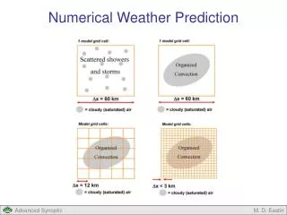
Forecast Quality Forecast quality is a function of grid spacing/feature resolution (more grid points are better) Forecasts using 2 times more grid points in each direction requires 16 times more processing power!!!
The Goal Use the maximum number of grid points Obtain a computationally bound model Result: produce better forecasts faster!
Tools Code analysis: Count arrays – assess memory requirements Calculations Data reuse etc Solution techniques (spatial and time differencing methods Use PAPI (Performance Application Programming Interface)to track FLOPS/cache misses etc Define metrics for evaluating solution techniques and predict results
Metrics Single precision flop to memory bandwidth ratio peak flop rating/peak main memory bandwidth Actual bandwidth needed to achieve peak flop rate (simple multiply: a = b*c) 4bytes/variable*3variables/flop*flops/clock*clock/sec Flops needed to cover the time required to load data from memory #of 3-D arrays *4bytes/array * required peak flop bandwidth
Research Weather Model 61 3-D arrays (including 11 temporary arrays (ARPS/WRF has ~150 3-D arrays) 1200 flops per/cell/iteration (1 big/small step) 3-time levels required for time dependant variables Split-time steps Big time step (temperature, advection, mixing) Small time step (winds, pressure) Result: ~5% of peak performance…
Solution Approach Compute computational and turbulent mixing terms for all variables except pressure Compute advection forcing for all variables Compute pressure gradient and update variables
Weather Model Equations (PDE’s) U,V,W represent winds Theta represents temperature Pi represents pressure T – Time X – east west direction Y – north south direction Z – vertical direction Turb – turbulence terms (what can’t be measured/predicted) S – Source terms, condensation, evaporation, heating, cooling D – numerical smoothing f – Coriolisforce (earth’s rotation)
Code Analysis Results Memory usage: 3 time levels for each predicted variable 11 temporary arrays (1/5 of the memory) Solution process breaks calculations up into several sections Compute one term thru the entire grid and then compute the next term Tiling can help improve the cache reuse but did not make a big difference
Previous Results Cache misses were significant Need to reduce cache misses via: Reduction in overall memory requirements Increase operations per memory reference Simplify the code (if possible)
Think outside the box Recipe: Not getting acceptable results? (~5% peak) Develop useful metrics Check the compiler options Other numerical solution methods Using simple loops to achieve peak performance on an instrumented platform Then apply the results to the full scale model
Revised Code New time scheme to reduce memory footprint (RK3, no time splitting!) Reduces memory requirements by 1 3-D array per time dependant variable (reduces footprint by 8 arrays) More accurate (3rd order vs 1st order) Combine ALL computations into one loop (or directional loops) Removes need for 11 temporary arrays
Weather Model Equations (PDE’s) U,V,W represent winds Theta represents temperature Pi represents pressure T – Time X – east west direction Y – north south direction Z – vertical direction Turb – turbulence terms (what can’t be measured/predicted) S – Source terms, condensation, evaporation, heating, cooling D – numerical smoothing f – Coriolisforce (earth’s rotation)
Revised Solution Technique Reuses data Reduces intermediate results and loads to/from memory Sample loops:
2nd Order U-Velocity Update call PAPIF_flops(real_time, cpu_time, fp_ins, mflops, ierr) DO k=2,nz-2 ! scalar limits u(2) is the q's/forcing. DO j=2,ny-1 ! scalar limits u(1) is the ! updated/previous u DO i=2,nx-1 ! vector limits u(i,j,k,2)=-u(i,j,k,2)*rk_constant c e-w adv : -tema*((u(i+1,j,k,1)+u(i,j,k,1))* : (u(i+1,j,k,1)-u(i,j,k,1)) : + (u(i,j,k,1)+u(i-1,j,k,1))* (u(i,j,k,1)-u(i-1,j,k,1))) c n-s adv : -temb*((v(i,j+1,k,1)+v(i-1,j+1,k,1))* : (u(i,j+1,k,1)-u(i,j,k,1)) : + (v(i,j,k,1)+v(i-1,j,k,1))* (u(i,j,k,1)-u(i,j-1,k,1))) c vert adv : -temc*((w(i,j,k+1,1)+w(i-1,j,k+1,1))* : (u(i,j,k+1,1)-u(i,j,k,1)) : + (w(i,j,k,1)+w(i-1,j,k,1))*(u(i,j,k,1)-u(i,j,k-1,1))) c pressure gradient : -temd*(ptrho(i,j,k)+ptrho(i-1,j,k))* : (pprt(i,j,k,1)-pprt(i-1,j,k,1)) c compute the second order cmix x terms. : + temg*(((u(i+1,j,k,1)-ubar(i+1,j,k))- : (u(i,j,k,1)-ubar(i,j,k)))- : ((u(i,j,k,1)-ubar(i,j,k))- (u(i-1,j,k,1)-ubar(i-1,j,k)))) ontinuedL c compute the second order cmix y terms. • : + temh*(((u(i,j+1,k,1)-ubar(i,j+1,k))- • : (u(i,j,k,1)-ubar(i,j,k)))- • : ((u(i,j,k,1)-ubar(i,j,k))- • : (u(i,j-1,k,1)-ubar(i,j-1,k)))) • c compute the second order cmix z terms. • : + temi*(((u(i,j,k+1,1)-ubar(i,j,k+1))- • : (u(i,j,k,1)-ubar(i,j,k)))- • : ((u(i,j,k,1)-ubar(i,j,k))- • : (u(i,j,k-1,1)-ubar(i,j,k-1)))) • END DO ! 60 calculations... • END DO • END DO • call PAPIF_flops(real_time, cpu_time, fp_ins, mflops, ierr) • print *,'2nd order u' • write (*,101) nx, ny,nz, • + real_time, cpu_time, fp_ins, mflops 60 flops/7 arrays
4th order U-Velocity uadv/mix call PAPIF_flops(real_time, cpu_time, fp_ins, mflops, ierr) DO k=2,nz-2 ! scalar limits u(2) is the q's/forcing. DO j=2,ny-2 ! scalar limits u(1) is the updated/previous u DO i=3,nx-2 u(i,j,k,2)=-u(i,j,k,2)*rk_constant1(n) c e-w adv : -tema*((u(i,j,k,1)+u(i+2,j,k,1))*(u(i+2,j,k,1)-u(i,j,k,1)) : +(u(i,j,k,1)+u(i-2,j,k,1))*(u(i,j,k,1)-u(i-2,j,k,1))) : +temb*((u(i+1,j,k,1)+u(i,j,k,1))*(u(i+1,j,k,1)-u(i,j,k,1)) : + (u(i,j,k,1)+u(i-1,j,k,1))*(u(i,j,k,1)-u(i-1,j,k,1))) : -tema*(((((u(i+2,j,k,1)-ubar(i+2,j,k))-(u(i+1,j,k,1)-ubar(i+1,j,k)))- : ((u(i+1,j,k,1)-ubar(i+1,j,k))-(u(i,j,k,1)-ubar(i,j,k))))- : (((u(i+1,j,k,1)-ubar(i+1,j,k))-(u(i,j,k,1)-ubar(i,j,k)))- : ((u(i,j,k,1)-ubar(i,j,k))-(u(i-1,j,k,1)-ubar(i-1,j,k)))))- : ((((u(i+1,j,k,1)-ubar(i+1,j,k))-(u(i,j,k,1)-ubar(i,j,k)))- : ((u(i,j,k,1)-ubar(i,j,k))-(u(i-1,j,k,1)-ubar(i-1,j,k))))- : (((u(i,j,k,1)-ubar(i,j,k))- (u(i-1,j,k,1)-ubar(i-1,j,k)))- : ((u(i-1,j,k,1)-ubar(i-1,j,k))-(u(i-2,j,k,1)-ubar(i-2,j,k)))))) END DO’s Print PAPI results… 52 flops/3 arrays
4th order W wadv/mix Computation call PAPIF_flops(real_time, cpu_time, fp_ins, mflops, ierr) DO k=3,nz-2 ! limits 3,nz-2 DO j=1,ny-1 DO i=1,nx-1 w(i,j,k,2)=w(i,j,k,2) c vert adv fourth order : +tema*((w(i,j,k,1)+w(i,j,k+2,1))*(w(i,j,k+2,1)-w(i,j,k,1)) : +(w(i,j,k-2,1)+w(i,j,k,1))*(w(i,j,k,1)-w(i,j,k-2,1))) : -temb*((w(i,j,k-1,1)+w(i,j,k,1))*(w(i,j,k,1)-w(i,j,k-1,1)) : +(w(i,j,k+1,1)+w(i,j,k,1))*(w(i,j,k+1,1)-w(i,j,k,1))) c compute the fourth order cmix z terms. : -tema*((((w(i,j,k+2,1)-w(i,j,k+1,1))- : (w(i,j,k+1,1)-w(i,j,k,1)))- : ((w(i,j,k+1,1)-w(i,j,k,1))- (w(i,j,k,1)-w(i,j,k-1,1))))- : (((w(i,j,k+1,1)-w(i,j,k,1))-(w(i,j,k,1)-w(i,j,k-1,1)))- : ((w(i,j,k,1)-w(i,j,k-1,1))-(w(i,j,k-1,1)-w(i,j,k-2,1))))) END DO ! 35 calculations... END DO END DO call PAPIF_flops(real_time, cpu_time, fp_ins, mflops, ierr) print *,'wadvz' write (*,101) nx, ny,nz, + real_time, cpu_time, fp_ins, mflops 35 flops/2 arrays
Final U Loop call PAPIF_flops(real_time, cpu_time, fp_ins, mflops, ierr) DO k=2,nz-2 ! complete the u computations DO j=2,ny-2 DO i=2,nx-1 u(i,j,k,1) = u(i,j,k,1) + u(i,j,k,2)*rk_constant2(n) END DO END DO END DO call PAPIF_flops(real_time, cpu_time, fp_ins, mflops, ierr) print *,'ufinal' write (*,101) nx,ny,nz, + real_time, cpu_time, fp_ins, mflops 2 flops/2 arrays
Individual Loop Tests Hardwired array bounds (due to PGI compiler 3.2 version not optimizing when using dynamic array allocation) Prefetching must be specified Varied array sizes/memory footprint Use 3 loops from 2nd and 4th order (spatial) solution techniques Compare flops/timings/metrics
Memory size = 5 arrays *4* nx*ny*nz Chicago = P3 Laptop
Model Tests Current scheme (Klemp-Wilhelmson method) 2nd and 4th order spatial differencing RK3 scheme: all computations (except temperature) are computed on the small time step (6x more work is performed in this case as in the current scheme) Show results from various platforms as a function of mflops and percent of peak
Test Setup 5 sec dtbig, 0.5 sec dtsmall 1000x1000x250m grid spacing 600 second warm bubble simulation No turbulence (ok for building scale flow predictions!) Dry dynamics only
Flop Count/per Iteration 4th Order: Current code: 1200 flops (all terms) ~600 flops for these tests Revised code: ~535 flops (w/o terrain, moisture) 2nd Order: 260 flops (w/o terrain, moisture)
Summary Notable improvement in % of peak from reduced memory footprint Longer vector lengths are better BUT: RK3 (revised) method still requires more wall clock time (>50%) for a single core, tests are underway to see if this is the case when using multiple cores Apply this method to the adv/mixing part of the existing code to improve performance (e.g. loop result) Recommendation: Apply higher order numerics to achieve higher % of peak (almost free)
Multi-Core Tests Compared current and revised (reduced memory requirement and revised order of computations) weather model MPI versions Timings for 1,2,4,8 cores per node on Sooner (OU Xeon-based Supercomputer) Sooner has two chips/node with 4 cores/chip Zero-slope line is perfect scaling
Multi-Core Results Discussion Contention for the memory bus extends application run time 2 cores/node is approximately 90% efficient (2-10% overhead due to 2 cores accessing memory) 4 cores/node produces 25-75% overhead 8 cores/node produces 243-417% overhead (> 2-4 x slower than 1 processor test) – but doing 8x more work
Multi-Core Summary Multi-core performance scales very well at 2 cores/node but scalability is drastically reduced when using 8 cores/node Contention for memory becomes significant for memory intensive codes at 8 cores/node (OU Sooner HPC system)
Credits: • Dr. Henry Neeman (OSCER) • Scott Hill (OU-CAPS PAPI) • PSC (David ONeal) • NCSA • Tinker AFB