Download
1 / 27
270 likes | 405 Views
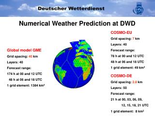
CCAM Numerical Weather Prediction. Dr Marcus Thatcher Research Scientist December 2007. Overview. Numerical Weather Prediction with CCAM Example: Processing NCEP GFS analyses Indonesia 60 km resolution 8 day forecast Jakarta 8 km resolution 4 day forecast

E N D
CCAM Numerical Weather Prediction Dr Marcus Thatcher Research Scientist December 2007
Overview • Numerical Weather Prediction with CCAM • Example: • Processing NCEP GFS analyses • Indonesia 60 km resolution 8 day forecast • Jakarta 8 km resolution 4 day forecast • Bali 8 km resolution 4 day forecast • Post processing forecast output CMAR NWP
Overview • CCAM NWP forecasts are constructed in two stages • The first stage creates a 60 km forecast for 8 days into the future • The second stage downscales the 60 km forecast to 8 km resolution. Normally this is only done for 3 days into the future CMAR NWP
CCAM uses nudging to ‘step down’ the forecast resolution from 60km 8km 1km. Downscaling Initial forecast 60km Nudging 8km Nudging 1km CMAR NWP
GFS analysis Summary of the CCAM system Initial conditions Data Products (web pages, etc) CCAM Local terrain and vegetation User latitude/ longitude CMAR NWP
GFS analysis Summary of the CCAM system Initial conditions CCAM 60km forecast Extract forecast data Topography and vegetation Data Products (web pages, etc) Downscaling CCAM 8km forecast Extract forecast data User latitude/ longitude Topography and vegetation Downscaling CCAM 1km forecast Extract forecast data Topography and vegetation CMAR NWP
CCAM NWP Example • The scripts for the CCAM NWP example are located under: • $HOME/ccam/scripts/nwp • The script that runs the simulation is called: • startforecast.sh CMAR NWP
The startforecast.sh script performs four main functions: Downloads NCEP GFS analyses and processes the analysis for initial conditions Runs a 60 km resolution forecast for Indonesia Runs two 8 km forecasts that are nested in the 60 km forecast (Jakarta and Bali as examples) Processes the output from CCAM so that it can be used CCAM NWP Example Download and prepare IC Run 60 km forecast 8 km forecast 8 km forecast Process model output CMAR NWP
1) Downloading initial conditions • CCAM can use various analysis products for initial conditions, including: • NCEP GFS 0.5 deg • NCEP GFS 1 deg • Australian BoM GASP 1 deg • CMC 1 deg • NOGAPS 1 deg • For this example we will use the NCEP GFS analysis CMAR NWP
Summary: NCEP GFS analysis is downloaded using getanalysis.sh Process the GRIB file using procgfs2.sh CCAM initial conditions are then located in $HOME/ccam/scripts/nwp/obs/avn CCAM initial conditions can be inspected using GrADS or Ferret 1) Downloading initial conditions Download analysis (getanalysis.sh) Process GRIB (procgfs2.sh) CCAM initial conditions CMAR NWP
Next, the CCAM 60 km resolution forecast is run. The runall script simply starts the Indonesian forecast if the last forecast is older than the analysis jog48indon contains all the information needed to run CCAM 2) 60 km resolution forecast Start forecasts (runall) Indonesia 60 km forecast (jog48indon) CMAR NWP
jog48indon converts the initial conditions to a conformal cubic (CC) grid using cdfvidar Soil initial conditions are generated using smclim from a soil climatology dataset. It is also possible to use soil data from the last forecast. Pre-generated topography and land-use datasets are located in the ~/ccam/scripts/data directory 2) 60 km resolution forecast Convert initial conditions to CC (cdfvidar) Prepare soil initial conditions (smclim) Topography and land-use CMAR NWP
Then CCAM namelist file (called input) is prepared Some example CCAM namelist switches are provided dt = time step (20mins) nwt = output interval ntau = total number of steps kdate_s = start date ktime_s = start time leap = use leap year? io_in = interpolate initial conditions from input? mfix = mass conservation mfix_qg = moisture conservation 2) 60 km resolution forecast CMAR NWP
ifile = intial conditions file mesonest = boundary conditions file albfile = albedo file zofile = roughness file rsmfile = rsmin file vegfile = vegetation file (SiB) soilfile = soil data file (Zobler) ofile = CCAM output file 2) 60 km resolution forecast CMAR NWP
After running CCAM, we need to convert the output back to a regular grid using cc2hist Different output variables can be specified in the cc2hist namelist It is also possible to obtain the output in pressure levels 2) 60 km forecast Run CCAM (globpea.q1) Process output (cc2hist) CMAR NWP
3) cc2hist – processing CCAM output • A typical cc2hist command looks like: • cc2hist –r 0.5 ccout.nc llout.nc < cc.nml • Where • -r determines the output resolution in deg • ccout.nc is the CCAM output (on the CC grid) • llout.nc is the CCAM output converted to a regular grid • cc.nml is the namelist that specifies the output variables and the output domain. • Instructions for cc2hist can be obtained by: • cc2hist -h CMAR NWP
3) cc2hist – processing CCAM output • Below is an example cc2hist namelist &input kta=0, ktb=99999, ktc=-1 minlat = -20., maxlat = -10., minlon = 90., maxlon = 120. use_plevs = T plevs = 1000, 900, 800, 700, 600, 500, 400, 300, 200 &end &histnl hnames = "temp","u","v","psl","rnd24","tscrn","zs","mixr","zg","tmaxscr","tminscr" hfreq = 1, htype = "inst", hbytes=2 &end Output all timesteps Output domain Use and define Pressure levels (instead of sigma levels) Output variables (also just use “all”) CMAR NWP
3) cc2hist – processing CCAM output • CCAM output from the 60 km forecast can be found at • $HOME/ccam/scripts/nwp/save/indon-0701/indon_60km • Once processed by cc2hist, we can examine the CCAM NWP forecast using GrADS or Ferret • It is also possible to examine the ‘raw’ CCAM 60 km forecast on the conformal cubic grid • $HOME/ccam/scripts/nwp/wdir/indon/indon_60km • By looking at the ‘raw’ output shows what variables you can process with cc2hist CMAR NWP
Once the 60 km forecast is complete, we can downscale to 8 km resolution forecast for multiple locations For example, here we downscale to 8 km resolution forecasts for Jakarta and Bali As before, the output is controlled by cc2hist 4) 8 km nested forecasts 60 km Indonesian forecast (jog48indon) 8 km Bali forecast (jog48bali) 8 km Jakarta forecast (jog48jaka) CMAR NWP
For nested forecasts, the CCAM namelist is slightly different mesonest = CCAM 60 km output filename io_in = -1 to interpolate the 60km BC to the 8km CC grid dt = 3 mins nbd = -3 (far field nudging) nud_uv = nudge winds nud_p = nudge surface pressure nud_t = nudge temperature nud_q = nudge mixing ratio nud_hrs = efolding time kbotdav = lowest model level to nudge (1 = all levels) 4) 8 km nested forecasts CMAR NWP
Sigma levels kbotdav=4 (typically NWP) kbotdav=10 (typically climate) CMAR NWP
5) cc2hist – processing 8 km CCAM output • CCAM output from the 8 km forecast can be found at • $HOME/ccam/scripts/nwp/save/indon-0701/jaka_8km • $HOME/ccam/scripts/nwp/save/indon-0701/bali_8km • The ‘raw’ CCAM 8 km forecast on the conformal cubic grid is located at • $HOME/ccam/scripts/nwp/wdir/indon/jaka_8km • $HOME/ccam/scripts/nwp/wdir/indon/bali_8km CMAR NWP
CCAM output • Typically the forecast is stored in • 3 hour (60km) or • 1 hour (8km) intervals. • This is because the radiation scheme is normally updated once every hour. • The default areas of the forecast are: • 60km ±15deg ~ ±1700kms • 8km ±2deg ~ ±220kms • 1km ±0.25deg ~ ±30kms • Since CCAM is a global model, the output can be also global. However, usually the output is for the high resolution cubic panel only CMAR NWP
CCAM output Typical output area CMAR NWP
GFS analysis Example forecast system GFS download and archive system Data integrity system Generator for client data products Operational forecasting system Hindcast system CCAM Validation and verification system Archive and synchronization with parallel forecast systems Delivery platform (web pages, FTP, etc) Data store CMAR NWP
Thank You Contact CSIRO Phone 1300 363 400 +61 3 9545 2176 Email enquiries@csiro.au Web www.csiro.au Marine and Atmospheric Research Name Dr Marcus Thatcher Title Research Scientist Email Marcus.Thatcher@csiro.au