Download
1 / 17
260 likes | 495 Views
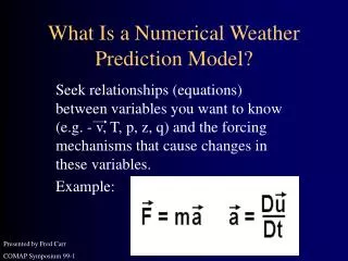
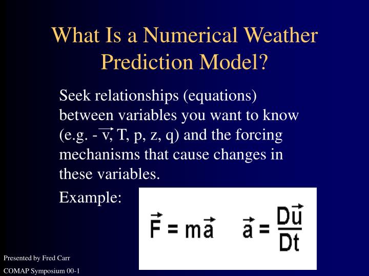
What Is a Numerical Weather Prediction Model?. Seek relationships (equations) between variables you want to know (e.g. - v, T, p, z, q) and the forcing mechanisms that cause changes in these variables. Example:. Presented by Fred Carr COMAP Symposium 00-1. In meteorology, we solve for Du/Dt

E N D
What Is a Numerical Weather Prediction Model? Seek relationships (equations) between variables you want to know (e.g. - v, T, p, z, q) and the forcing mechanisms that cause changes in these variables. Example: Presented by Fred Carr COMAP Symposium 00-1
Or or Example of a prognostic equation
Example of a diagnostic equation: Just consider vertical component of (1): rhs balances perfectly for large-scale flow: Hydrostatic eq. - used to deduce Z from T
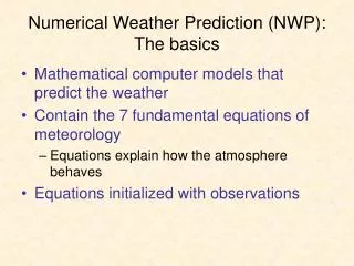
Thus, the essential components of an NWP model are: 1. Physical Processes - RHS of equations (e.g., PGF, friction, adiabatic & diabatic heating (advection terms are also on rhs unless have Lagrangian model)
2. Numerical Procedures approximations used to estimate each RHS term (especially imp. for advection terms) approximations used to integrate model forward in time grid used over model domain (resolution) boundary conditions Note: Quality and quantity of observations (initial conditions) equally vital to NWP system Need to observe prognostic variables
Primitive Equation Models A. Primitive Equations It was recognized early in the history of NWP (Charney, 1955) that the primitive equations of motion would be best suited for development of comprehensive dynamical-physical models of the atmosphere. Although the problems of initialization and numerical integration of the primitive equations are still areas of research, stable forecasts from these equations have been produced for over 35 years.
We will present the primitive equations in x-y-p coordinates and discuss some general properties of this system. These equations are equally appropriate for global as well as limited-area models. A set of governing equations that describe large-scale atmospheric motions can be derived from conservation laws governing momentum, mass, energy, and moisture (see Holton, 1979 - Chap. 2). These are called the primitive
equations, not because they are crude or simplistic but because they are fundamental or basic. Using the Eulerian framework in x-y-p coordinates, they can be written as follows: (1) (2) (3) (4) (5) (6)
Eqs. (1) and (2) are the horizontal momentum equations for the u- and v- components of the wind, respectively. Note that (via scale analysis), the curvature terms and the 2cos Coriolis term have been neglected. Eq. (3) is the vertical momentum equation under the assumption of hydrostatic balance (diagnoses z). The continuity equation (4) expresses the conservation of mass (diagnoses w). The First Law of Thermodynamics yields an “energy” equation for temperature (5). Eq. (6) is the conservation of moisture equation where q is specific humidity.
The dependent variables in this set of equations are u, v, , , T, and q which are assumed to be continuous functions of the independent variables x, y, p, and t. Eqs. (1), (2), (5), and (6) are prognostic equations (involve a time derivative) and thus require initial conditions. Initial conditions are derived from observations or the use of some balance relationship (e.g. - obtaining u and v from by assuming geostrophic balance). Eqs. (3) and (4) are diagnostic equations and can be computed once the initial conditions are provided. Thus, (1) to (6) constitute a set of 6 equations in 6 unknowns
and we can say we have a closed system if: i) we can find expressions for Fx, Fy, H, E, and P in terms of the known dependent variables ii) we have suitable initial conditions over the domain iii) suitable lateral boundary conditions for the dependent variables are formulated (for regional models); all models need boundary conditions at the top and bottom levels
The first category above encompasses the whole subject of adding “physics” to the primitive equations. Fx and Fy are “friction” terms which modify the momentum equations via surface drag (skin friction) and horizontal and vertical transport of momentum by turbulent eddies of various sizes (generally called diffusion in large-scale models). The diabatic heating term H also consists of several effects which can be written H = HL + HC + HR + HS (7)
where HL is due to latent heat of condensation caused by the large-scale dynamic ascent of stably-stratified, saturated air (grid-scale precipitation), HC is the latent heat rate due to convection (cumulus parameterization), HR is the radiative heating rate and HS represents sensible heat flux from the surface of the earth. One of the most difficult problems in NWP is how to formulate proper expressions for the net effects of HC, HR, and HS (which are generally subgrid-scale processes) in terms of the large-scale dependent variables (the parameterization problem). The precipitation rate P=PL+PC is known once HL and HC are known.
Evaporation E can be due to moisture flux from the surface and evaporation of precipitation. The effect of mountains also has to be included in the model via the lower boundary condition and choice of vertical coordinate . Once conditions (i) to (iii) are “suitably“ met (the fact that they are never perfectly met accounts for a large part of the total forecast error), the equations (1) to (6) can, in principle, be solved in the following straightforward manner:
1. Obtain observations of the prognostic variables u, v, T, and q over the domain 2. Compute from (3) and from (4) 3. Compute Fx, Fy, H, E, P and the other terms on the right-hand sides of (1), (2), (5), and (6) 4. Integrate the four prognostic equations forward in time to obtain new values of u, v, T, and q 5. Repeat steps 2 to 4 until complete the forecast
Since there are nearly an infinite number of ways to formulate the physics and many numerical procedures are available for the solution of the equations, no two numerical models are alike. Thus each model may have systematic errors or biases peculiar to itself. However, some errors, such as those arising from insufficient resolution, are common to all models. It is important for forecasters to become aware of these limitations in order to make “Intelligent Use of Model Guidance”.