Download
1 / 49
490 likes | 626 Views
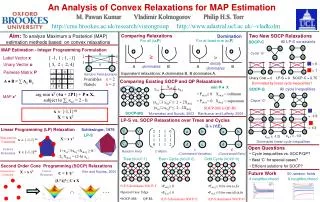
Efficiently Solving Convex Relaxations. for MAP Estimation. M. Pawan Kumar University of Oxford. Philip Torr Oxford Brookes University. Aim. To solve convex relaxations of MAP estimation. 0. 6. 1. 3. 2. 0. 4. Label ‘1’. 1. 2. 4. 1. 1. 3. Label ‘0’. 1. 0. 5. 0. 3. 7. 2.

E N D
Efficiently Solving Convex Relaxations for MAP Estimation M. Pawan Kumar University of Oxford Philip Torr Oxford Brookes University
Aim • To solve convex relaxations of MAP estimation 0 6 1 3 2 0 4 Label ‘1’ 1 2 4 1 1 3 Label ‘0’ 1 0 5 0 3 7 2 b c d a Random Variables V = {a, b, c, d} Edges E = {(a, b), (b, c), (c, d)} Label Set L = {0, 1} Labelling m = {1, 0, 0, 1}
Aim • To solve convex relaxations of MAP estimation 0 6 1 3 2 0 4 Label ‘1’ 1 2 4 1 1 3 Label ‘0’ 1 0 5 0 3 7 2 b c d a Cost(m) = 2 + 1 + 2 + 1 + 3 + 1 + 3 = 13 Minimum Cost Labelling? NP-hard problem Approximate using Convex Relaxations
Aim • To solve convex relaxations of MAP estimation 0 6 1 3 2 0 4 Label ‘1’ 1 2 4 1 1 3 Label ‘0’ 1 0 5 0 3 7 2 b c d a Objectives • Solve tighter convex relaxations – LP and SOCP • Handle large number of random variables, e.g. image pixels
Outline • Integer Programming Formulation • Linear Programming Relaxation • Additional Constraints • Solving the Convex Relaxations • Results and Conclusions
Cost of a = 1 Cost of a = 0 Integer Programming Formulation 2 0 4 Unary Cost Label ‘1’ 1 3 Label ‘0’ 5 0 2 b a Labelling m = {1 , 0} ; 2 4 ] 2 Unary Cost Vector u = [ 5
a = 1 a 0 Integer Programming Formulation 2 0 4 Unary Cost Label ‘1’ 1 3 Label ‘0’ 5 0 2 b a Labelling m = {1 , 0} ; 2 4 ]T 2 Unary Cost Vector u = [ 5 Label vector x = [ -1 1 ; 1 -1 ]T Recall that the aim is to find the optimal x
Integer Programming Formulation 2 0 4 Unary Cost Label ‘1’ 1 3 Label ‘0’ 5 0 2 b a Labelling m = {1 , 0} ; 2 4 ]T 2 Unary Cost Vector u = [ 5 Label vector x = [ -1 1 ; 1 -1 ]T 1 Sum of Unary Costs = ∑iui (1 + xi) 2
Pairwise Cost Matrix P 0 0 Cost of a = 0 and b = 0 0 0 1 0 Cost of a = 0 and b = 1 0 1 0 0 3 0 0 0 Integer Programming Formulation 2 0 4 Pairwise Cost Label ‘1’ 1 3 Label ‘0’ 5 0 2 b a Labelling m = {1 , 0} Pairwise Cost of a and a 3 0
Pairwise Cost Matrix P 0 0 0 1 0 0 1 0 0 3 0 0 0 Integer Programming Formulation 2 0 4 Pairwise Cost Label ‘1’ 1 3 Label ‘0’ 5 0 2 b a Labelling m = {1 , 0} Sum of Pairwise Costs 1 ∑ijPij (1 + xi)(1+xj) 0 3 0 4
Pairwise Cost Matrix P 0 0 0 1 0 1 = ∑ijPij (1 + xi + xj + Xij) 4 0 1 0 0 3 0 0 0 Integer Programming Formulation 2 0 4 Pairwise Cost Label ‘1’ 1 3 Label ‘0’ 5 0 2 b a Labelling m = {1 , 0} Sum of Pairwise Costs 1 ∑ijPij (1 + xi +xj + xixj) 0 3 0 4 X = x xT Xij = xi xj
Uniqueness Constraint ∑ xi = 2 - |L| i a Integer Programming Formulation Constraints • Integer Constraints xi{-1,1} X = x xT
∑ xi = 2 - |L| i a Non-Convex Integer Programming Formulation 1 1 ∑ Pij (1 + xi + xj + Xij) x* = argmin + ∑ ui (1 + xi) 4 2 Convex xi{-1,1} X = x xT
Outline • Integer Programming Formulation • Linear Programming Relaxation • Additional Constraints • Solving the Convex Relaxations • Results and Conclusions
∑ xi = 2 - |L| i a Linear Programming Relaxation Schlesinger, 1976 Retain Convex Part 1 1 ∑ Pij (1 + xi + xj + Xij) x* = argmin + ∑ ui (1 + xi) 4 2 xi{-1,1} X = x xT
∑ xi = 2 - |L| i a ∑ Xij = (2 - |L|) xi j b Linear Programming Relaxation Schlesinger, 1976 Retain Convex Part 1 1 ∑ Pij (1 + xi + xj + Xij) x* = argmin + ∑ ui (1 + xi) 4 2 xi[-1,1] Xij[-1,1] 1 + xi + xj + Xij≥ 0
Dual of the LP Relaxation Wainwright et al., 2001 1 1 a b c a b c 2 d e f 2 d e f 3 g h i 3 g h i 4 5 6 = (u, P) a b c d e f g h i ii 4 5 6
Dual of the LP Relaxation Wainwright et al., 2001 1 Q(1) a b c a b c d e f 2 Q(2) d e f g h i 3 Q(3) g h i Q(4) Q(5) Q(6) = (u, P) a b c Dual of LP d e f max i Q(i) g h i ii 4 5 6
Tree-Reweighted Message Passing Kolmogorov, 2005 4 5 6 a b c a b c 1 Pick a variable a 2 d e f d e f g h i g h i 3 u2 u4 u1 u3 c b a a d g Reparameterize such that ui are min-marginals Only one pass of belief propagation
Tree-Reweighted Message Passing Kolmogorov, 2005 4 5 6 a b c a b c 1 Pick a variable a 2 d e f d e f g h i g h i 3 (u2+u4)/2 (u2+u4)/2 (u1+u3)/2 (u1+u3)/2 c b a a d g Average the unary costs TRW-S Repeat for all variables
Outline • Integer Programming Formulation • Linear Programming Relaxation • Additional Constraints • Solving the Convex Relaxations • Results and Conclusions
a d e Cycle Inequalities Chopra and Rao, 1991 a b c d e f At least two of them have the same sign xi xixj xjxk xkxi xj xk Xij Xjk Xki X = xxT At least one of them is 1 Xij + Xjk + Xki -1
xl xi b c xj xk e f Cycle Inequalities Chopra and Rao, 1991 a b c d e f Xij + Xjk + Xkl - Xli -2 Generalizes to all cycles LP-C
xi 1 Xij Xik xc = Xc = xj Xij 1 Xjk Xc xcxcT xk Xik Xjk 1 Second-Order Cone Constraints Kumar et al., 2007 a b c d e f Xc = xcxcT 1 • (Xc - xcxcT) 0 SOCP-C (xi+xj+xk)2 ≤ 3 + Xij + Xjk + Xki
xi 1 Xij Xik Xil xc = Xc = xj Xij 1 Xjk Xjl xk Xik Xjk 1 Xkl xl Xil Xjl Xkl 1 Second-Order Cone Constraints Kumar et al., 2007 a b c d e f SOCP-Q 1 • (Xc - xcxcT) 0
Outline • Integer Programming Formulation • Linear Programming Relaxation • Additional Constraints • Solving the Convex Relaxations • Results and Conclusions
a b c 1 a d g 4 2 5 d e f b e h g h i 3 c f i 6 1 2 a b b c max i Q(i) d e e f ii 3 4 d e e f g h h i Modifying the Dual a b c d e f g h i + j sj + j sj
Modifying TRW-S a b b c a b c a d g d e e f d e f b e h d e e f g h i c f i g h h i Pick a variable --- a Pick a cycle/clique with a REPEAT max i Q(i) + j sj ii Can be solved efficiently + j sj Run TRW-S for trees with a
Properties of the Algorithm Algorithm satisfies the reparametrization constraint Value of dual never decreases CONVERGENCE Solution satisfies Weak Tree Agreement (WTA) WTA not sufficient for convergence More accurate results than TRW-S
Outline • Integer Programming Formulation • Linear Programming Relaxation • Additional Constraints • Solving the Convex Relaxations • Results and Conclusions
4-Neighbourhood MRF Test SOCP-C Test LP-C 50 binary MRFs of size 30x30 u≈ N (0,1) P≈ N (0,σ2)
4-Neighbourhood MRF σ = 5 LP-C dominates SOCP-C
8-Neighbourhood MRF Test SOCP-Q 50 binary MRFs of size 30x30 u≈ N (0,1) P≈ N (0,σ2)
8-Neighbourhood MRF σ = 5 /2 SOCP-Q dominates LP-C
Conclusions • Modified LP dual to include more constraints • Extended TRW-S to solve tighter dual • Experiments show improvement • More results in the poster
Future Work • More efficient subroutines for solving cycles/cliques • Using more accurate LP solvers - proximal projections • Analysis of SOCP-C vs. LP-C
Timings Linear in the number of variables!!
Video Segmentation Keyframe User Segmentation Segment remaining video ….
Video Segmentation Input Belief Propagation 8175 25620 18314
Video Segmentation Input -swap 1187 1368 1289
Video Segmentation Input -expansion 2453 1266 1225
Video Segmentation Input TRW-S 6425 1309 297
Video Segmentation Input LP-C 719 264 294
Video Segmentation Input SOCP-Q 0 0 0
4-Neighbourhood MRF σ = 1
4-Neighbourhood MRF σ = 2.5
8-Neighbourhood MRF σ = 1/2
8-Neighbourhood MRF σ = 2.5 /2