Download
1 / 1
10 likes | 98 Views
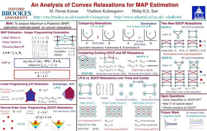
An Analysis of Convex Relaxations for MAP Estimation. Aim: To analyze Maximum a Posteriori (MAP) estimation methods based on convex relaxations. Comparing Relaxations. Two New SOCP Relaxations. Domination. For all ( u , P ). For at least one ( u , P ). All LP-S constraints. SOCP-C. a.

E N D
An Analysis of Convex Relaxations for MAP Estimation Aim:To analyze Maximum a Posteriori (MAP) estimation methods based on convex relaxations Comparing Relaxations Two New SOCP Relaxations Domination For all (u,P) For at least one (u,P) All LP-S constraints SOCP-C a b a b MAP Estimation - Integer Programming Formulation Cycle ‘G’ 0 ≥ > 4 2 [ -1, 1 ; 1, -1] c d Label Vector x c 3 1 2 5 strictly dominates [ 5, 2 ; 2, 4] = 0 Unary Vector u 0 dominates A A B B Vb Va = 1 Pairwise Matrix P a b b c c a Equivalent relaxations: A dominates B, B dominates A. Random Field Example Unary Cost = 0 LP-S = 0 SOCP-C = 0.75 #variables n = 2 #labels h = 2 AB = ∑ Aij Bij Comparing Existing SOCP and QP Relaxations Dominated by linear cycle inequalities? Xab;ij min P X xa;i xb;j All cycle inequalities SOCP-Q Xab;ij = infimum arg min xT (4u + 2P1) + P X, subject to ∑i xa;i = 2 - h x {-1,1}nh X = xxT • Pab;ij ≥ 0 a b a b MAP x* Xab;ij = supremum • Pab;ij < 0 Clique ‘G’ (xa;i+ xb;j)2 ≤ 2 + 2Xab;ij c d c (xa;i- xb;j)2 ≤ 2 - 2Xab;ij SOCP-MS is QP-RL SOCP-MS Muramatsu and Suzuki, 2003 Ravikumar and Lafferty, 2006 = -1/3 a b b c c d LP-S vs. SOCP Relaxations over Trees and Cycles G = (V,E) = 1/3 Linear Programming (LP) Relaxation Schlesinger, 1976 Va Vb a b a b 2 1 1 0 d a a c b d LP-S 1 2 1 1 xa;1 = -1/3 xa;0 = -1/3 Non-convex Constraint X = xxT x {-1,1}nh 1 1 2 1 Dominates linear cycle inequalities Vd Vc d c d c 0 1 1 2 Open Questions Convex Relaxation V (Constrained Variables) E (Constrained Pairs) 1+xa;i+xb;j+Xab;ij ≥ 0 Random Field C Matrix x [-1,1]nh • Cycle inequalities vs. SOCP/QP? j Xab;ij = (2-h) xa;i Tree (SOCP-T) Even Cycle (SOCP-E) Odd Cycle (SOCP-O) • Best ‘C’ for special cases? Second Order Cone Programming (SOCP) Relaxations • Efficient solutions for SOCP? Non-convex Constraint X = xxT Convex Relaxation Kim and Kojima, 2000 Future Work C = U UT 50 random fields 4 neighbourhood 8 neighbourhood ||UTx||2≤ C X • LP-S dominates SOCP-T • Pab;ij ≥ 0 • Pab;ij ≥ 0 for one (a,b) … • Special Case: Edge • Pab;ij ≤ 0 • Pab;ij ≤ 0 for one/all (a,b) • SOCP-MS/ QP-RL • LP-S dominates SOCP-E • LP-S dominates SOCP-O