Download
1 / 39
1.54k likes | 3.14k Views
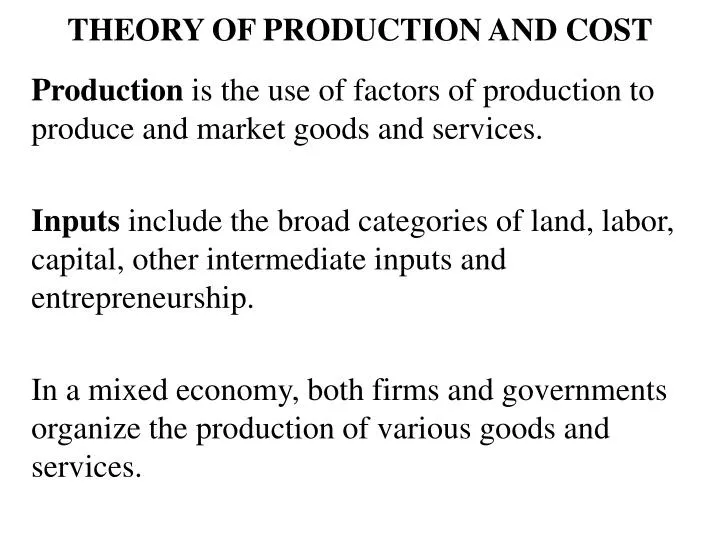
THEORY OF PRODUCTION AND COST. Production is the use of factors of production to produce and market goods and services. Inputs include the broad categories of land, labor, capital, other intermediate inputs and entrepreneurship.

E N D
THEORY OF PRODUCTION AND COST Production is the use of factors of production to produce and market goods and services. Inputs include the broad categories of land, labor, capital, other intermediate inputs and entrepreneurship. In a mixed economy, both firms and governments organize the production of various goods and services.
Production in the Short-run An input that cannot vary in quantity during the relevant time period is called a fixed input or fixed factor. An input having a quantity that can change during the relevant time period is called a variable input or variable factor. The short-run is a period of time such that there is at least one fixed factor. The long-run is a period of time such that all inputs are variable in quantity.
A production function summarizes the relationship between all combinations of inputs and the corresponding maximum attainable levels of output, for a given technology. The total product, TP, of a variable input is the amount of output produced over the period when that input is used with fixed quantities of all other inputs. The marginal productof an input F, MPF, is the additional output per unit increase in the input, holding all other inputs (and technology) constant;
Diminishing marginal product: As more of a variable input is employed, with the quantities of all other inputs held constant, the marginal product of the variable input will decline after some point. Diminishing marginal product results from the process of adding additional units of a variable input to given quantities of other inputs.
Measuring costs and profits Total (Economic) Cost is the monetary value of all inputs used in a particular activity over a given period. Explicit Costs correspond to the monetary payments for inputs. Implicit Costs are the opportunity costs of inputs that have no explicit monetary payments as a result of the inputs not being purchased in markets. All opportunity costs, both explicit and implicit, are part of economic costs.
Measuring costs Economic depreciation is the reduction in the value of a capital good over the relevant period that results from wear and tear as well as obsolescence. Accounting depreciation measures the annual accounting cost of capital, expressed as some portion of the capital’s monetary cost. Accounting costs measure the explicit costs of production during a given period plus accounting depreciation.
Measuring costs and profits Total revenue is the explicit monetary return associated with an economic activity over a given period. Economic activities can also yield implicit returns. The total return includes both total revenues and implicit returns.
Economic and accounting profits are defined below: Total return Total revenue less: less: explicit costs explicit costs economic depreciation accounting depreciation other implicit costs Economic ProfitsAccounting Profits Economic profits measure the net (private) economic gain resulting from an economic activity. When economic profits are zero the returns to owner supplied inputs exactly equal the opportunity costs of those inputs. These returns are called normal profits.
Related Cost Measures Variable cost, VC, is the cost of the variable input(s) used to produce any given level of output. Fixed costs, FC, is the cost of all fixed inputs. Total cost, TC, is the sum of the costs of all inputs used to produce output during the period; TC = VC + FC.
Example of Potato Production (The price of fertilizer is $50 per unit and the costs associated with fixed input $40.)
Related Cost Measures Marginal cost, MC, is the increase in total or variable cost per unit increase in output, Q;
Average variable cost, AVC, is the variable cost of production per unit of output; Average fixed cost, AFC, is the fixed cost per unit of output; Average cost, AC, is the total cost of all inputs per unit of output;
1.43 103
2.33 1.94 0.39 103
For example, if MPL= 0.5 widgets per hour and the wage rate is a constant $10.00 per hour, MC = ($10 per hour) / (0.5 widgets per hour) = $20 per widget . Intuition: If MPL= 0.5, it takes two hours of work to create one widget. With a wage of $10 per hour, this translates into a marginal cost of $20.00 for an additional widget. The marginal cost of output directly depends upon the marginal product and price of each variable input;
Implications: • An increase in the price of a variable input, ceteris paribus, will result in an increase in the marginal cost of output. • Holding the input price constant, an increase in the marginal product of a variable input will cause MC to decrease. • Often we talk about MC increasing as output increases (after some point). The underlying reason is diminishing marginal product of the variable input(s).
MC = 1.90 MC = 0.70 MC = 1.30 ΔTC = 0.70 ΔQ = 1 Total-Cost Curve...(Another Example) $16.00 Total-cost curve $14.00 $12.00 $10.00 Total Cost $8.00 $6.00 $4.00 $2.00 $0.00 2 4 6 8 10 12 0 Quantity of Output
MC AVC Average-Cost and Marginal-Cost Curves... $3.50 $3.00 $2.50 $2.00 Costs $1.50 $1.00 $0.50 $0.00 2 4 6 8 10 12 0 Quantity of Output
Relationship Between Marginal Cost and Average Variable Cost • Whenever MC is greater than AVC, AVC will be rising. • Whenever MC is less than AVC, AVC will be falling.
MC ATC Relationship Between Marginal Cost and Average Total Cost $3.50 $3.00 $2.50 $2.00 Costs $1.50 $1.00 $0.50 $0.00 0 2 4 6 8 10 12 Quantity of Output
Relationship Between Marginal Cost and Average Total Cost • Whenever MC is less than ATC, ATC will be falling. • Whenever MC is greater than ATC, ATC will be rising.
MC ATC AVC AFC Average-Cost and Marginal-Cost Curves... $3.50 $3.00 $2.50 $2.00 Costs $1.50 $1.00 $0.50 $0.00 2 4 6 8 10 12 0 Quantity of Output
Cost Curves and Their Shapes The average total-cost curve is U-shaped. • At very low levels of output ATC is high because fixed cost is spread over only a few units. • ATC initially declines as output increases because of the decline in AFC. • ATC eventually starts to rise because AVC rises substantially.
Total-Cost Curve... $16.00 Total-cost curve $14.00 $12.00 $10.00 Total Cost $8.00 $6.00 $4.00 $2.00 $0.00 2 4 6 8 10 12 0 Quantity of Output
Big Bob’s Cost Curves... $20.00 $18.00 Total Cost Curve $16.00 $14.00 $12.00 Total Cost $10.00 $8.00 $6.00 $4.00 $2.00 $0.00 0 2 4 6 8 10 12 14 16 Quantity of Output (bagels per hour)
MC AVC Big Bob’s Cost Curves... 3.5 3 2.5 2 Costs 1.5 1 0.5 0 0 2 4 6 8 10 12 14 16 Quantity of Output
MC AVC AFC Big Bob’s Cost Curves... 3.5 3 2.5 2 Costs 1.5 1 0.5 0 0 2 4 6 8 10 12 14 16 Quantity of Output
MC ATC AVC AFC Big Bob’s Cost Curves... 3.5 3 2.5 2 Costs 1.5 1 0.5 0 0 2 4 6 8 10 12 14 16 Quantity of Output
Three Important Properties of Cost Curves: • Marginal cost eventually rises with the quantity of output. • The average-total-cost curve is U-shaped. • The marginal-cost curve crosses the average-total-cost and average-variable-cost curves at their minimums.
Cost Curves and Their Shapes The bottom of the U-shape AC curve corresponds to the quantity that minimizes the average cost of production. This quantity is sometimes called the efficient scale of the firm. The marginal-cost curve crosses the average-total-cost curve at the efficient scale.
Costs in the Long Run • For many firms, the division of total costs between fixed and variable costs depends on the time horizon being considered. • In the short run some costs are fixed. • In the long run fixed costs become variable costs.
ATC in short run with small factory ATC in short run with medium factory ATC in short run with large factory ATC in long run Average Total Cost in the Short and Long Runs... Average Total Cost 0 Quantity of Cars per Day
Economies and Diseconomies of Scale • Economies of scale occur when long-run average total cost declines as output increases. • Diseconomies of scale occur when long-run average total cost rises as output increases. • Constant returns to scale occur when long-run average total cost does not vary as output increases.
ATC in long run Economies of scale Constant Returns to scale Diseconomies of scale Economies and Diseconomies of Scale Average Total Cost 0 Quantity of Cars per Day