Download
1 / 45
450 likes | 566 Views
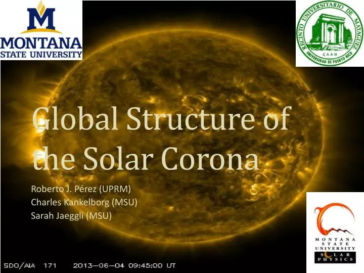
Global Structure of the Solar Corona. Roberto J. Pérez (UPRM) Charles Kankelborg (MSU) Sarah Jaeggli (MSU). Abstract.

E N D
Global Structure of the Solar Corona Roberto J. Pérez (UPRM) Charles Kankelborg (MSU) Sarah Jaeggli (MSU)
Abstract • The AIA instrument on the Solar Dynamics Observatory obtains images of the sun in seven different extreme ultraviolet wavebands. Each filter produces images with distinctive appearance that is apparent to experienced observers. Subjective descriptions abound in the literature and in conference presentations, as do qualitative explanations of the physical reasons for these differences. We seek a quantitative description of the image properties, with the aim of understanding what the general image properties indicate about the temperature structure of the corona. Our preliminary results, obtained at multiple heliocentric angles above and below the limb, show that some channels consistently present a high or low intensity contrast which we attribute to the differing temperature, density and filling factor of the structures imaged. We also investigate the power spectra characteristic of each waveband.
Main Question • Why are images produced by different EUV (Extreme ultraviolet) filters so different? Can these differences be caused by physical parameters or could it be that different filters image specific solar structures?
Possible Explanations • Some papers present qualitative explanations • Instrument Scattering, Resonance Scattering and contamination of photons in the passbands has been suggested but they have been proven wrong. • “Filling-Factor Model” – Piling up of structures along the line of sight
Data • SDO (Solar Dynamics Observatory) (NASA) - AIA (Atmospheric Image Assembly) • We consider seven different EUV (Extreme Ultraviolet) wavebands. • 94 Angstroms • 131 Angstroms • 171 Angstroms • 193 Angstroms • 211 Angstroms • 304 Angstroms • 335 Angstroms
Approach • Extract intensity arrays corresponding to different heliocentric annular regions. • 2^14 elements • Divide the arrays by their median value (For means of comparison) • Compare these arrays using different techniques
Histograms • The histograms presented here were created by taking the average of histograms corresponding to twelve consecutive Carrington rotations of the sun (roughly). • The frequency axis is log-scaled
Observations • High frequency of low intensity pixels in the 335 and 94 wavebands • Relatively similar structure among wavebands • Seemingly erratic behavior far above the solar limb.
Contrast • We define contrast as the difference between the 75th percentile intensity value and the 25th percentile value.
Observations • 94, 335, and 211 consistently have the higher contrast in all annular regions. • This does not support our initial hypothesis that the images that look less “fuzzier” to our eyes (ie. 304) should have the higher contrast. • The 304 waveband consistently presents a low contrast. • The plots from annular regions below the limb look different from the ones above the limb. Imaging of different ionic species could be an explanation for this.
Contrast vs. Characteristic Temperature • It is possible to deduce a characteristic temperature for each waveband. • This does not mean that everything imaged in that waveband is at that specific temperature but it provides a nice approximation. • Some ions are only imaged in specific solar activities (ie. Flares). For our purposes we use the most stable temperature that corresponds to each waveband.
Observations • For annular regions below the limb we can observe a light correlation between characteristic temperature and contrast. • Annular regions above the solar limb show no correlation at all. • It is important to note that the waveband that has the lowest characteristic temperature almost always has the lowest contrast below the limb while the waveband that has the highest characteristic temperature almost always presents the highest contrast below the limb. • 304 is dominated by Si XI (Log(6.2)=6.2) above the limb.
Discrete Fourier Transforms • These plots consist of the average of Fourier transform plots corresponding to twelve consecutive Carrington rotations of the sun. • The intensity component axis is log scaled • The frequency axis is presented as log(frequency) • The frequency axis goes to the Nyquist frequency
Observations • Linear behavior below the limbs (small bumps noticeable in the 94, 304 and 131 wavebands. • Bumps become more noticeable above the limbs • Could the bumps be of solar origin? • Mean Signal (335-94-131-304) : Bump height (94-335-131-304) (Highest to lowest) • Period of some solar structures: • Sunspots: ~33 arcsecs • Granules: ~1.4-2.0 arcsecs (frequency range: (-1.7) – (-0.15)) • Supergranules: ~49 arcsecs • Coronal Holes: ~974-1252 arcsecs • Active Region Loops: ~14 arcsecs • Spicules: ~.7 arcsecs
Overall Results • The characteristic temperature of a specific waveband seems to have an effect on the contrast observed. • The temperature of the imaged structure of each waveband appears to directly affect the contrast or ‘fuzziness” that our eyes perceive. • It is possible that some temporary solar structures are affecting the overall consistency of the results (This needs further proof) • The bumps on the Fourier transform plots seem to be of solar origin. Granular and supergranular scales look relevant. • Hotter wavebands present bumps (Coronal heating problem?)
Further Work • Construction of a coronal model - Densities of the solar structures imaged - Temperature map of the plasma imaged by the different wavebands Find the origin of the bumps on the Fourier transform plots.
References • The Transparency of Solar Coronal Active Regions (Brickhouse & Shmelz, 2005) • Warm And Fuzzy: Temperature and Density Analysis of an Fe XV EUV Imaging Spectrometer Loop (Shmelz et al., 2011) • Are Coronal Loops Isothermal or Multithermal? (Shmelz et al., 2009) • SDO/AIA Response to Coronal Hole, Quiet Sun, Active Region and Flare Plasma (O’Dwyer et al. , 2010)