Download

1 / 22
230 likes | 423 Views
Magnetic Field Maps of the Solar Corona. Haosheng Lin, Jeffrey R. Kuhn, & Roy Coulter Institute for Astronomy, University of Hawaii. ABSTRACT

E N D
Magnetic Field Maps of the Solar Corona Haosheng Lin, Jeffrey R. Kuhn, & Roy Coulter Institute for Astronomy, University of Hawaii • ABSTRACT • A longstanding problem for understanding the solar corona has been to measure the magnetic field that we believe determines its structure and dynamics from the upper chromosphere out into the heliospheric environment. Despite a long history of optical measurements it is only recently that Zeeman splitting observations of infrared coronal emission lines (Lin et al. 2000) have been used to successfully deduce the coronal magnetic flux density. Here we extend this technique and report first results from a novel coronal magnetometer that uses an off-axis reflecting coronagraph (SOLARC) and optical fiber-bundle imaging spectropolarimeter (OFIS). Our results reveal the line-of-sight magnetic flux density with a sensitivity of a few gauss with 20 arcsec spatial resolution and approximately 60min temporal resolution. These full Stokes spectropolarimetric measurements of the forbidden FeXIII 1075nm emission line reveal the line-of-sight coronal magnetic field 100" above an active region to have a flux density of about 5G. We also measured the orientation of the magnetic fields projected in the plane of the sky. These two-dimensional magnetic field maps of the solar corona -- coronal magnetograms-- will yield valuable information to further our understanding of the solar corona. SHINE 2004, Big Sky, Montana
Coronal Magnetic Field—Our Dark Energy Problem • The coronal magnetic field is something of a "dark energy'' problem for us in that we know it permeates the corona and controls its static and dynamic behavior, yet we are unable to usefully measure it. There are no tools for remotely sensing coronal magnetic fields except for occasional sight-lines to background radio sources suitable for Faraday rotation measurements (Stelzerid 1970). Perhaps radio (e.g. gyrosynchrotron) magnetometry techniques will become generally useful for inferring stronger active region field strengths low in the corona (Gary & Hurford, 1994), but these techniques are still developing. Determining the magnetic field along an arbitrary coronal line-of-sight is clearly a difficult observational problem but here we demonstrate significant progress toward this goal with sensitive imaging spectropolarimetric observations of the IR forbidden coronal emission line of FeXIII at a wavelength of 1075nm. • It has been known since the first quantitative observations of the infrared coronal emission lines of FeXIII at 1075nm and 1080nm by Firor and Zirin (1962) that these lines have important diagnostic potential for determining physical conditions of the coronal plasma near a temperature of 2MK. Chevalier and Lambert (1969) and Flower and des Forets (1973) described the exquisite sensitivity of the IR FeXIII lines to the local electron density. Somewhat later House (1977) showed with detailed line formation calculations, and Querfeld (1977) with observations, how the linear polarization of the 1075nm line could be used to determine the coronal magnetic field orientation. SHINE 2004, Big Sky, Montana
History of Coronal B Observations • Harvey, 1969: Fe IV 530 nm Stokes V magnetometry No definitive detection. • Mickey, 1973: Fe IV 530 nm Stokes Q and U polarimetry • Successfully obtained maps of the orientation of coronal magnetic fields. • Querfeld, and Smartt, 1984: Fe XIII 1075 nm Stokes Q and U polarimetry • Successfully obtained maps of the orientation of coronal magnetic fields • Arnaud & Newkird, 1987: Fe XIII 1075 nm Stokes Q and U polarimetry • Successfully obtained maps of the orientation of coronal magnetic fields • Kuhn, 1995: Fe XIII 1075 nm Stokes Vspectropolarimetry No definitive detection. • Lin, Penn, & Tomczyk, 2000: Fe XIII 1075 nm Stokes V spectropolarimetry • Definitive detection of line-of-sight coronal magnetic field! SHINE 2004, Big Sky, Montana
Example of Coronal Emission Line Spectropolarimetry, October 25, 1999 • Weak Stokes V signals from the FeXIII 1074.7 nm line are measurable! SHINE 2004, Big Sky, Montana
Definitive Stokes V Signal • NSO/SP Evans Solar Facilities 40 cm coronagraph • 240 arcsec FOV (summed over the entire length of the slit). • 2560 seconds (44 minutes) integration time. • Careful telescope and instrumental polarization cross-talk control SHINE 2004, Big Sky, Montana
Can We Make 2-D Coronal Magnetic Field Maps? IfA Coronal B Initiatives • While Lin et al. (2000) demonstrated the feasibility of using CEL polarimetry to measure the strength of coronal magnetic fields, useful measurements require 2-dimensional spatial coverage. To this goal, IfA scientists initiated a new effort to establish the capability to make 2-dimensional maps of both longitudinal magnetic field strength and the orientation of the magnetic field projected in the plane of the sky. • The IfA effort includes: • Construction of a 50 cm aperture off-axis mirror coronagraph—SOLARC • Construction of an Optical Fiber-bundle Imaging Spectropolarimeter (OFIS) SHINE 2004, Big Sky, Montana
SOLARC: Off-Axis Mirror Coronagraph SOLARC and its dome on the summit of Haleakala, Maui. SOLARC is a 50 cm aperture off-axis mirror coronagraph. A field stop located at its prime focus serves as an inverse occulter to select the coronal target region and reject the glaring photospheric radiation. The FOV (field-of-view) of the telescope is approximately 400 arcsec in diameter. A LCVR-based (Liquid Crystal Variable Retarder) polarimeter at the gregorian focus analyzes the polarization of the CEL before the fiber optics bundle. Secondary mirror Prime focus inverse occulter/field stop Re-imaging lens LCVR Polarimeter Input array of fiber optics bundle Primary mirror SHINE 2004, Big Sky, Montana
OFIS: Optical Fiber-Bundle Imaging Spectropolarimeter Echelle Grating Camera Lens Collimator NICMOS3 IR camera Fiber Bundle • The spectrograph of OFIS is a bench-mounted spectrograph. It is equipped with: • NICMOS3 IR Camera • 16 8 => 2 64 fiber optics integral field unit • 160 308 mm, 79 lines/mm echelle grating with 63.5 blaze angle • f = 800 mm, = 150 mm (F/5.3) collimator and camera lens The coherent optical fiber-bundle rearrange the 2-dimensional image sampled by the 16 × 8 input array to two linear array (2 × 64 ). The two linear arrays act as the slits of the spectrograph, thus allowing for the simultaneous recording of the spectra from all the field points in the 2-D image plane. SHINE 2004, Big Sky, Montana
Sample CEL Spectra from OFIS One column illuminated 16 × 4 pixels area coverage Two columns illuminated 16 × 8 pixels area coverage SHINE 2004, Big Sky, Montana
2004/04/06 Observation • Full Stokes vector observations were obtained on April 6, 2004 on active region NOAA 0581 during its west limb transit. • Stokes I, Q, U, & V Observation: • 20arcsec/pixel resolution • Telescope pointing @ • Radius Vector 0.25 R • Position Angle (Geocentric): 260°. • 70 minutes integration on V • 15 minutes integration on Q & U • Stokes I, Q & U Scan: • RV = 0.25 R • From PAG 250° to 270° • Five 5° steps Fe X 171Å image of the solar corona at approximately the time of SOLARC/OFIS observation from the Extreme Ultraviolet Imaging Telescope of the Solar and Heliospheric Observatory (EIT/SOHO). The rectangle marks the target region of the coronal magnetic field (Stokes V) observation. SHINE 2004, Big Sky, Montana
Full Stokes Spectra of CEL • Stokes I, Q, U, and V images obtained from active region NOAA 0581during its west limb transit. The spectra are arranged in order such that each 16-fiber strip (0 to 15, 16 to 31, etc.) in the vertical direction corresponds to a 16-fiber row along the east-west direction in increasing height, i.e., the lowest 16-fiber strip (0 to 15) corresponds to the row furthest south. • The Stokes I spectra were flatfielded by a ‘sky flat’ taken at 1.75 solar radii above quiet Sun. Due to the scattering of photospheric light off the atmosphere of the Earth and telescope optics, absorption lines can also be seen in these spectra images. The Fraunhofer line at 1074.4 nm to the left of the Fe XIII line is a Si I line. The Stokes V spectra in the CEL image does not show the characteristic anti-symmetrical profiles of magnetic field induced circular polarization. • Instead, its spectral profiles are similar to that of the Stokes I (and Q and U). Furthermore, its spatial variation appears to be similar to that of the Stokes U spectral image. It is therefore apparent that there is substantial linear-to-circular polarization crosstalk in these data. The display ranges for I, Q, U, and V are -0.5 IC to 0.5 IC, -0.05 IC to 0.05 IC, -0.05 IC to 0.05 IC, and -0.005 IC to 0.005 IC, respectively. SHINE 2004, Big Sky, Montana
Polarization Crosstalk Correction • Due to the high temperature and low magnetic field strength of the corona, The circular polarization of the CEL is expected to be below 1 × 10⁻³IL (line intensity). On the other hand, the magnitude of linear polarization is expected to be on the order of 1 × 10⁻¹IL. Thus, even a very small linear-to-circular polarization crosstalk is sufficient to produce the observed intensity-like Stokes V profiles. • The crosstalk contaminated circular polarization V’ ()can be expressed by • V’ = V + a ·Q + b ·U = V + ·I, • where V () is the uncontaminated circular polarization signal, a and b are the Q-V and U-V crosstalk coefficients, respectively, and is an ‘apparent’ I-V crosstalk coefficient. Using a least squares algorithm minimizing • 2 = (V’ – V - ·I), • we can derived assuming I ·V=0 due to the antisymmetric property of V, • = I ·V’ / I 2. Row Stokes V and crosstalk-corrected V. The image is rearranged such that the each 8-fiber strip in the vertical direction corresponds to a 8-fiber column in the north-south direction. The first 8 rows (0-7) correspond the column closest to the solar limb. The weak antisymmetric V profiles can be seen in the first two north-south columns (fiber 0 to 16) in the crosstalk-corrected V image. Alternative, since in weak-field approximation, V = B·dI/d, the observed circular polarization can be written as _V’ () = ·I () + B ·dI () /d = ·I (+ B/), Thus, B can be directly measured by comparison with the shift of V with respect to I in the spectral direction. The two methods give statistically identical magnetic field measurements. SHINE 2004, Big Sky, Montana
Polarimetric Diagnostics of Coronal B • Linear Polarization • Orientation of CEL linear polarization maps the orientation of magnetic field projected in the plane-of-sky (POS). • Orientation of linear polarization is subject to the Van Vleck 90 degrees ambiguity. • Circular Polarization • Circular polarization of CEL is proportional to the strength of line-of-sight magnetic field • The magnetograph formula is modified by an alignment factor that depends on the inclination angle between B and the local vertical direction, and the anisotropy of the incident radiation field. SHINE 2004, Big Sky, Montana
Line-of-Sight Magnetic Fields B B Samples of measured and fitted Stokes I and V spectra of the 10 4 (200” 80”) pixel region closest to the solar limb. The errors of the magnetic fields are 1 sigma error. Geocentric north is up, and east is left. The longitudinal field reverses sign around h=0.17 R SHINE 2004, Big Sky, Montana
Transverse Field Orientation 1 • Does intensity loops track magnetic field lines? • Yes, and No! • See boxes 1 and 2 • Degree of polarization decreases as a function of height=> higher anisotropy and less collisional depolarization. • Van Vleck effect in box 2? 2 SHINE 2004, Big Sky, Montana
Transverse Field Orientation 1 • Does intensity loops track magnetic field lines? • Yes, and No! • See boxes 1 and 2 • Degree of polarization decreases as a function of height=> higher anisotropy and less collisional depolarization. • Van Vleck effect in box 2? 2 SHINE 2004, Big Sky, Montana
‘Vector’ Coronal Magnetogram Transverse field orientation Longitudinal Magnetic Fields Contour plot of the line-of-sight magnetogram over-plotted on the EIT FeXVI 284 A image. The contours are 5G, 3G, and 1G. SHINE 2004, Big Sky, Montana
Radial Variations of B and Comparison with Model Calculations Average B as a function of height from the limb from the center of the FOV. The solid line with errors plots the IR data. The dotted line shows the Abbett et al. (2003) near-limb "breakout" magnetic model scaled to an active region with 1000G longitudinal field strength at the photosphere. It doesn't extend high enough for a good comparison. The * with error bars are the global Ledvina et al. (2004) B model (rms field evaluated along averaged horizontal sight path). The upper error bars show the maximum field at given horizontal level, the lower error flag shows the standard deviation of the model B and the plotted symbols show the mean rms B at the given horizontal level. The observed unsigned field strength is qualitatively similar to that of the Ledvina B model. Averaged and fitted Stokes I & V spectra from the first 10 north-south columns used to construct the B radial variation plot. SHINE 2004, Big Sky, Montana
What Light’s Up Some Field Lines? – Is CEL Intensity Correlated with Magnetic Field Strength? • Magnetic fields fill the entire volume of the corona. However, intensity images of coronal emission lines always show highly distinctive loop structures. • Why some of the magnetic field lines are filled with high density highly ionized atoms, while the adjacent dark regions are not? • Are bright coronal loops actually representative of higher magnetic field strength regions? • Do they actually trace the magnetic field lines? Although we only measure the line-of-sight component of the magnetic field strength B, we can examine the correlation between |B| and the CEL intensity to get some idea about the relation between |B| and Iline. The scatter plot between |B| and Iline suggests that the bright CEL emission does not necessary imply stronger magnetic fields. SHINE 2004, Big Sky, Montana
Summary • We have successfully obtained the first coronal magnetogram, with measurements of both the longitudinal magnetic field strength and orientation of the magnetic field projected in the plane of the sky. The magnetic field sensitivity is ~ 1 G near the limb with approximately 1 hr integration with a 20” 20” spatial resolution. • We observed a radial fall-off of B qualitatively similar to that predicted by some numerical models. • We observed a non-radial magnetic field configuration similar to that implied by the EIT image. However, it is still not clear if the loop structures in the EIT image actually follow the magnetic field lines we measure in these FeXIII data. More studies are needed. • We find no correlation between the brightest emission structures and the strongest longitudinal magnetic fields SHINE 2004, Big Sky, Montana
What’s Next? • Data, lot’s of data! • Lot’s of data coordinated with other instruments! • Comparison with model calculations. • Vector Magnetogram? • Resolving line-of-sight integration problem--Tomography? • Larger aperture coronagraph and larger format OFIS will significantly improve the spatial resolution and coverage, time resolution, and magnetic field sensitivity of the observations. • Coronal magnetometry is photon starved – WE NEED A LARGER CORONAGRAPH – ATST? SHINE 2004, Big Sky, Montana