Download
1 / 59
590 likes | 680 Views
Observational data on Primary CR Spectrum. from here c = 1. CR composition at low energies. Particle abundances in CR (at E > 2.5 GeV/particle, minimum SA) and in Universe.

E N D
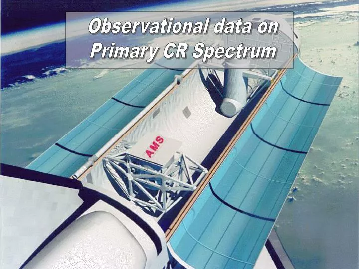
Observational data on Primary CR Spectrum
from here c = 1
CR composition at low energies Particle abundances in CR (at E > 2.5 GeV/particle, minimum SA) and in Universe The abundances of primary CR is essentially different from the standard abundances of nuclei in the Universe. The difference is biggest for the light nuclear groupL (Li, Be, B).
Over the charge region Z=1–28 (H–Ni), CR experiments in space can resolve the individual elements over an extended energy range. A summary of these data shows the relative abundance of CR at ~1 AU (solid line) along with the Solar System abundance (dashed line) for two different energy regimes, 70–280 MeV/nucleon and 1–2 GeV/nucleon. All abundances are normalized at one for silicium (Si) and the later is taken to be 100. [Reference: J.A. Simpson, Ann. Rev. Nucl. Part. Sci. 33 (1983) 323.]. CR abundance Normalization point • Hydrogen (H) and helium (He) are the dominant elements, constituting some 98% of the CR ions, but are still under-abundant in the CR relative to the Solar System abundance. • There is reasonably good agreement between the CR and Solar System abundance data for most of the even elements particularly for carbon (C), oxygen (O), magnesium (Mg) and iron (Fe). • The light elements lithium (Li), beryllium (Be) and boron (B) as well as scandium (Sc) and vanadium (V) in the sub-iron region are greatly over-abundant when compared to the Solar System abundance. This is a result of nuclearspallation in interstellar space by nuclei of higher charge. The secondary nuclei generated by these reactions with the interstellar gas will have essentially the same velocity as the incident primary nuclei and hence the same energy per nucleon. Their energy spectra tend to be steeper than those of the primaries due to energy-dependent escape of the higher-energy primaries from the Galaxy. Solar System abundance
The integral charge spectrum of CR nuclei. [Reference: E. Juliusso and P. Meyer, ApJ 201 (1975) 76.]
A BIRD'S EYE VIEW OF THE ALL-PARTICLE CR SPECTRUM Notes All nuclei Modulated by solar activity 1. The low’energy part of the spectrum (below some tens of GeV) is dependent of the geographycal position. 1 particle per m2×second ballons & satellites | | EAS experiments 2. Due to the presence of (at least) two knees this is probably not a human leg. Is it a leg of a bug? O the 2nd knee is a bug? Knee 1 particle per m2×year 2nd knee Ankle 1 particle per km2×year Foot (?) Fingers (?) Expected GZK cutoff
GZK ~ 5×10¹⁰ GeV 2nd knee ~ 4×10⁸ GeV 1st knee ~ 3×10⁶ GeV ankle ~ 5×10⁹ GeV
The Sun in short(photospheric features, sunspot cycle, etc.) Sun Facts Solar radius = 695,990 km = 109 Earth radii Solar mass = 1.989×1030 kg = 333,000 Earth masses Solar luminosity (energy output of the Sun) = 3.846×1033 erg/s Surface temperature = 5770 K = 10,400ºF Surface density = 2.07×10⁻⁷ g/cm3 = 1.6×10⁻⁴ Air density Surface composition = 70% H + 28% He + 2% (C, N, O, ...) by mass Central composition = 35% H + 63% He + 2% (C, N, O, ...) by mass Central temperature = 15,600,000 K = 28,000,000ºF Central density = 150 g/cm3 = 8 × Gold density Solar age = 4.57× 10⁹ yr
Sunspots Sunspotsappear as dark spots on the surface of the Sun. Temperatures in the dark centers of sunspots drop to about3700 K (compared to5700 Kfor the surrounding photo- sphere). They typically last for several days, although very large ones may live for several weeks. Sunspots are magnetic regions on the Sun with magnetic field strengths thousands of times stronger than the Earth's magnetic field. Sunspots usually come in groups with two sets of spots. One set will have positive or north magnetic field while the other set will have negative or south magnetic field. The field is strongest in the darker parts of the sunspots - theumbra. The field is weaker and more horizontal in the lighter part – thepenumbra.
Faculae: Faculae are bright areas that are usually most easily seen near the limb, or edge, of the solar disk. These are also magnetic areas but the magnetic field is concentrated in much smaller bundles than in sunspots. While the sunspots tend to make the Sun look darker, the faculae make it look brighter. During a sunspot cycle the faculae actually win out over the sunspots and make the Sun appear slightly (about 0.1%) brighter at sunspot maximum that at sunspot minimum.
Granules: Granules are small (about 1000 km across) cellular features that cover the entire Sun except for those areas covered by sunspots. These features are the tops of convection cells where hot fluid rises up from the interior in the bright areas, spreads out across the surface, cools and then sinks inward along the dark lanes. Individual granules last for only about 20 minutes. The granulation pattern is continually evolving as old granules are pushed aside by newly emerging ones. The flow within the granules can reach supersonic speeds of more than 7 km/s and produce sonic "booms" and other noise that generates waves on the Sun's surface. [The movie from Swedish Vacuum Solar Telescope.]
Supergranules: Supergranulesare much larger versions of granules(~ 35,000 kmacross) but are best seen in measurements of the Doppler shift where light from material moving toward us is shifted to the blue while light from material moving away from us is shifted to the red. These features also cover the entire Sun and are continually evolving. Individual supergranules last for a day or two and have flow speeds of about0.5 km/s. The fluid flows observed in supergranules carry magnetic field bundles to the edges of the cells where they produce the chromospheric network.
Animated Sun [Borrowed from Stanford Solar Center URL http://solar-center.stanford.edu/]. April-May 2003 April-May 2004 (last 30 days)
The Sunspot Cycle April, 2005 Monthly averages of the sunspot numbers show that the number of sunspots visible on the sun waxes and wanes with an approximate 11-year cycle. The figure is updated monthly by The Solar Physics Group at NASA's Marshall Space Flight Center [URL: http://science.nasa.gov/ssl/PAD/SOLAR/].
CR Neutron Monitoring (in short) The cosmic ray lab of University of Delaware at McMurdo Station, Ross Island, Antarctica. → University of New Hampshire cosmic ray labs at Huancayo, Peru (left) and Haleakala, Hawaii (right).
Low and intermediate energy part of the CR spectrum for the main nuclear groups
Primary differential kinetic-energy/nucleon spectra of CR protons and helium nuclei obtained near Earth near the solar minimum in 1965. [Reference: G. Gloeckler and J.P. Jokipi, ApJ 148 (1967) L41.]
Differential kinetic-energy spectra of protons in 1965, 1967, 1nd 1969. The 1965 spectrum is taken from the compilation of G. Gloeckler and J.P. Jokipi. [Reference: K.C. Hsieh et al., ApJ 166 (1971) 221.]
The proton(left panel) and helium(right panel) kinetic-energy spectra at the top of atmosphere detected by CAPRICE98 balloon-born experiment (marked by red circles) in comparison with several other, most recent experiments. [Reference: M. Boezio et al. (WiZard-CAPRICE98 Collaboration), Astropart. Phys. 19 (2003) , 583-604 (astro-ph/0212253).]
Flux spectra for downward going (a,b,c) and upward going (d,e,f) protons separated according to the geomagnetic latitude, QM, at which they were detected with AMS during the space shuttle flight STS-91 at an altitude of 380 km. [Reference:J. Alcaraz et al. (AMS Collaboration), Phys. Lett. B 472 (2000) 215-226 (hep-ex/0002049).]
CR proton (left panel) and helium (right panel) flux measurements are compared to the expected AMS-02. A two-phases cylindrical model of the Galaxy has been used to simulate the propagation of Protons and helium nuclei in the interstellar medium where they diffuse for roughly 2×10⁷ years. These nuclei are thedipest charged probes of the Galaxy since they diffuse on the average through one third of the Galactic disk and in the halo before being measured. [Reference:D. Casadei (for the AMS Collaboration), “Cosmic ray astrophysics with AMS-02,'‘ astro-ph/0404529.]
Isotopic Composition • Left panel: Kinetic-energy spectra of 1H and2H obtained from balloon and spacecraft (Voyager) • experiments at sunspot minimum modulation conditions in 1977. • Right panel: Kinetic-energy spectra of 3He and4He obtained from the same experiments. Estimated • magnitude of anomalous He component and galactic He are shown by dashed lines at low • energies. • In both panels, the data points designated by triangles are from Bastian et al. (1979) for a similar time • period. [Reference: W.R. Webber and S.M. Yushak, ApJ 275 (1983) 391.]
Left panel: The 3He/4He ratios measured as a function of kinetic energy in the balloon and spacecraft • experiments. Predictions of an interstellar propagation model for various values of the modulation • parameter are shown as solid lines. Corrections to the 3He/4He ratios for the presence of anomalous • 4He are shown by open and solid squares. • Right panel: Measured 2H/4He ratios at low energies and predictions based on the same interstellar • propagation model and local modulation as for He. Ratios corrected for anomalous 4He are shown • by open and solid squares at low energies. • [Reference: W.R. Webber and S.M. Yushak, ApJ 275 (1983) 391.]
The3He/4He ratios with measured in different experiments. The model predictions for various solar modulation levels are also shown with solid (φ = 0.35 GV), dashed (φ = 0.5 GV), dot line (φ = 1.0 GV), and dot-dashed (φ = 1.5 GV) lines. [Reference: Z. Xiong et al., JHEP 11 (2003) 048.] The dependence of average helium mass on the geomagnetic latitude measured with AMS. [Reference: Z. Xiong et al., JHEP 11 (2003) 048.]
AMS-02 expected performance on B/C ratio (left panel) after six months of data taking and 3He/4He ratio (right panel) after one-day of data taking compared to recent measurements. The B/C ratio was simulated according to a diffuse-reacceleration model (Strong & Moskalenko, 2001) with Alfvèn speed vA = 20 km/s, propagation region bounded by a galactocentric radius Rh = 30 kpc, distance from the galactic plane zh = 1 kpc. The 3He/4He ratio has been simulated according to the classical cosmic-ray transport Leaky Box Model with a rigidity dependent path-length distribution (Davis et al, 1995). [Reference:G. Lamanna, Mod. Phys. Lett. A 18 (2003) 1951-1966.]
Beryllium measurements. The expected AMS-02 1 year statistics is also shown assuming a model by Strong and Moskalenko. [Reference:D. Casadei (for the AMS Collaboration), “Cosmic ray astrophysics with AMS-02,'‘ astro-ph/0404529.]
Absolute flux [(m sr s TeV) -1 ] at E0 = 1 TeV/nucleus and spectral index of CR elements. Notes: (2) from PGM; (3) from B. Wiebel-Soth et al., Astron. Astrophys. 330 (1998) 389; (4) from PGM after an extrapolation for ultra-heavy elements.
Differential energy spectrum for protons. The best fit to the spectrum according to a power law is represented by the solid line, the bend (dotted line) is obtained from a fit to the all-particle spectrum. ← Differential energy spectrum for helium nuclei. The best fit to the spectrum according to a power law is represented by the solid line, the bend (dotted line) is obtained from a fit to the all-particle spectrum. ← Differential energy spectrum for iron nuclei. The best fit to the spectrum is represented by the solid line. ← Normalized all-particle energy spectra for individual experiments compared to one of the PGM. The individual results are shifted in steps of half a decade in flux in order to reduce overlap. In all 3 figures, the all-particle spectra are shown as dashed lines for reference.
All-particle energy spectra obtained from direct and indirect measurements. Normalized all-particle energy spectra for Individual experiments. In both figures, the sum spectra for individual elements according to the poly-gonato model are represented by the dotted line for 1≤ Z ≤ 28 and by the solid line for 1≤ Z ≤ 92. Above 108 GeV the dashed line reflects the average spectrum. Conclusion:The knee is explained as the subsequent cutoffs of the individual elements of the galactic component, starting with protons. The second knee seems to indicate the end of the stable elements of the galactic component.
Mean logarithmic mass vs. • primary energy. • Results from the average depth of the shower maximum Xmax using CORSIKA/QGSJET simulations. • Results from measurements of distributions for electrons, muons, and hadrons at ground level. Results from the balloon experiments JACEE and RUNJOB are given as well. Predictions according to the PGM are represented by the solid lines. The dashed lines are obtained by introducing an ad-hoc component of hydrogen only. Conclusion: The mass composition calculated with the PGM is in good agreement with results from EAS experiments measuring the electromagnetic, muonic and hadronic components at ground level. But the mass composition disagrees with results from experiments measuring the average depth of the shower maximum with Cherenkov and fluorescence detectors. If we believe the model we may conclude that <ln A> increases around and above the knee.
Comparison with several models from J. Candia, S. Mollerach and E. Roulet, JCAP 05 (2003) 003 [astro-ph/0302082]. The dotted straight line corresponds to an ad-hoc isotropic extragalactic component with a power-law spectrum.
A numerical solution to the Parker-Gleeson-Axford equation for modulated spectra of protons, electrons, and oxygen. The particles undergo a diffusive-like propagation in which trapping between time-varying constituents in the interplanetary magnetic field controls the particle motion. [Reference: L. Fisk, ApJ 206 (1976) 333.]
The positron fraction as a function of energy measured by CAPRICE98 (closed circles) and several other experiments. The dotted line is the secondary positron fraction calculated by R.J. Protheroe [ApJ 254 (1982) 391], the dashed and solid lines are the secondary positron fraction calculated by I.V. Moskalenko and A.W. Strong [ApJ 493 (1998) 694] with and without reacceleration of cosmic rays, respectively. [Reference: M. Boezio et al. (WiZard-CAPRICE98 Collaboration), ICRC’26, OG.1.1.16.]
Local interstellar e+/e-ratio measured by AMS-01 and CAPRICE94.
LIS of e+and e-measured by the most recent experiments plus high energy data from Nishimura et al. (1980), multiplied by E3.
LIS of e+and e- measured by all considered experiments, afterrenormalization to the AMS-01 and CAPRICE94 flux at 20 GeV, with a single power-law fit.